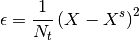
Contents
1. Data Structures
1.1. IO
1.1.1. CNOGraph
- class CNOGraph(model=None, data=None, verbose=False, **kargs)[source]
Data structure (Digraph) used to manipulate networks
The networks can represent for instance a protein interaction network (PIN).
CNOGraph is a data structure dedicated to the analysis of phosphorylation data within protein-protein interaction networks but can be used in a more general context. Note that CNOGraph inherits from the directed graph data structure of networkx.
- However, we impose links between nodes to be restricted to two types:
- “+” for activation
- “-” for inhibition.
An empty instance can be created as follows:
c = CNOGraph()
and edge can be added as follows:
c.add_edge("A", "B", link="+")
c.add_edge("A", "C", link="-")
An even simpler way is to add cno.io.reactions.Reaction, which can be strings or instance of the Reaction class.
The methods add_node() and add_edge() methods can be used to populate the graph. However, it is also possible to read a network stored in a file in cno.io.sif.SIF format:
>>> from cno import CNOGraph, cnodata
>>> pknmodel = cnodata("PKN-ToyPB.sif")
>>> c = CNOGraph(pknmodel)
The SIF model can be a filename, or an instance of SIF. Note for CellNOpt users that if and nodes are contained in the original SIF files, they are transformed int AND gates using “^” as the logical AND.
Other imports are available, in particular read_sbmlqual().
You can add or remove nodes/edges in the CNOGraph afterwards using NetworkX methods.
When instanciating a CNOGraph instance, you can also populate data from a XMIDAS data instance or a MIDAS filename. MIDAS file contains measurements made on proteins in various experimental conditions (stimuli and inhibitors). The names of the simuli, inhibitors and signals are used to color the nodes in the plotting function. However, the data itself is not used.
If you don’t use any MIDAS file as input, you can set the stimuli/inhibitors/signals manually by filling the hidden attributes _stimuli, _signals and _inhibitors with list of nodes contained in the graph.
Node and Edge attributes
The node and edge attributes can be accessed as follows (and changed):
>>> c.node['egf']
{'color': u'black',
 u'fillcolor': u'white',
 'penwidth': 2,
 u'shape': u'rectangle',
 u'style': u'filled,bold'}

>>> c.edge['egf']['egfr']
{u'arrowhead': u'normal',
 u'color': u'black',
 u'compressed': [],
 'link': u'+',
 u'penwidth': 1}
OPERATORS
CNOGraph is a data structure with useful operators (e.g. union). Note, however, that these operators are applied on the topology only (MIDAS information is ignored). For instance, you can add graphs with the + operator or check that there are identical
c1 = CNOGraph()
c1.add_reaction("A=B")
c2 = CNOGraph()
c2.add_reaction("A=C")
c3 = c1 +c2
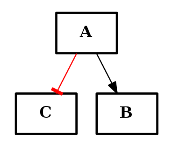
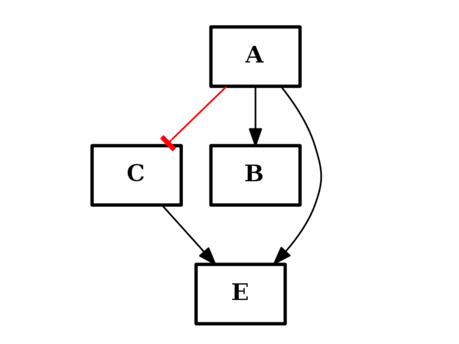
Let us illustrate the + operation with another example. Let us consider the following graphs:
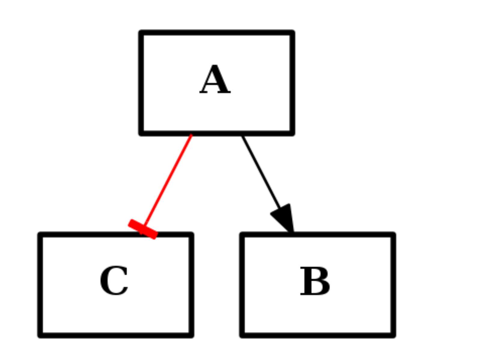
from cno import CNOGraph
c1 = CNOGraph()
c1.add_edge("A","B", link="+")
c1.add_edge("A","C", link="-")
c1.plot()
(Source code, png, hires.png, pdf)
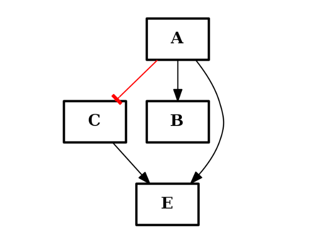
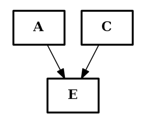
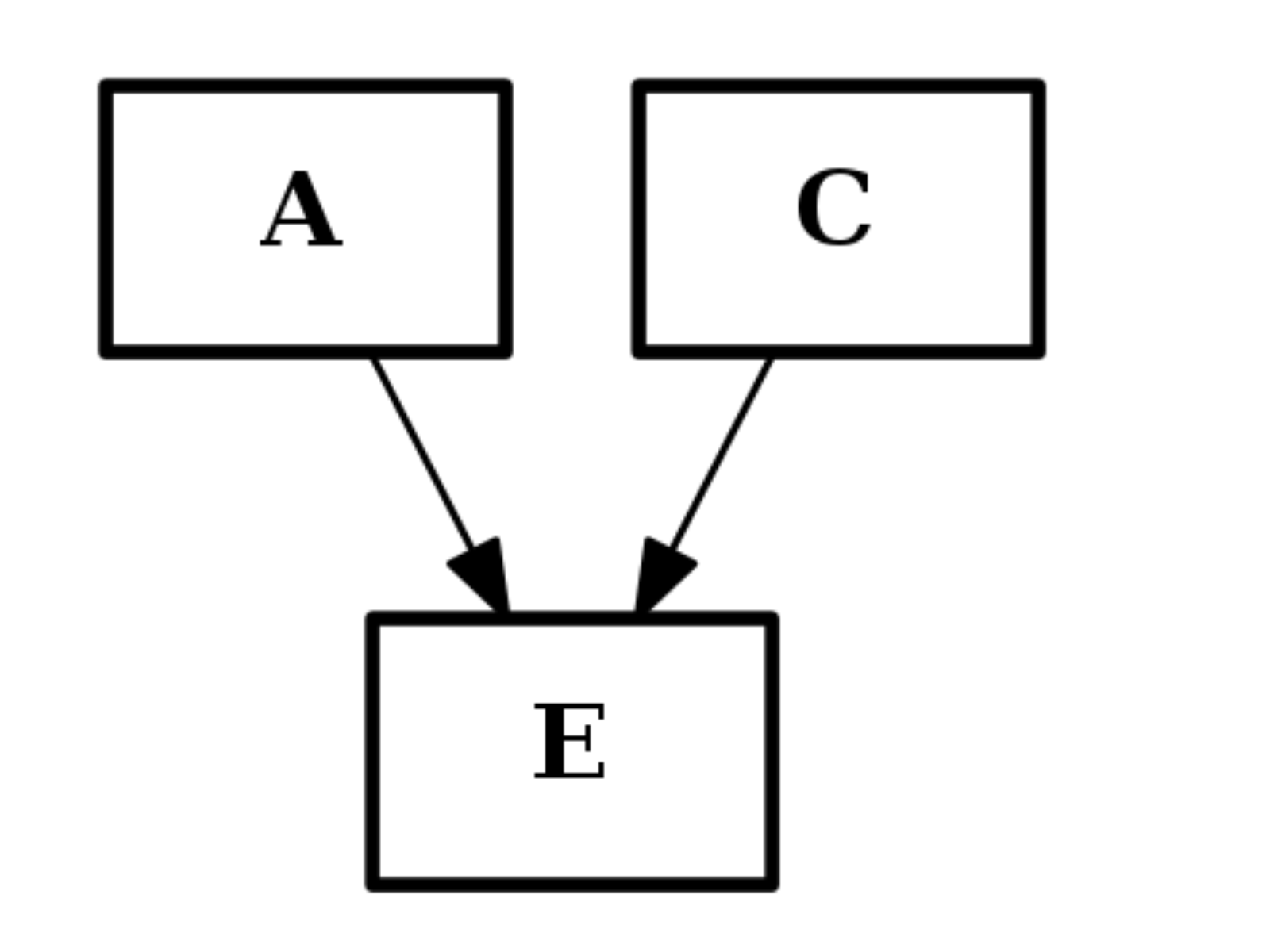
from cno import CNOGraph
c2 = CNOGraph()
c2.add_edge("A","E", link="+")
c2.add_edge("C","E", link="+")
c2.plot()
(Source code, png, hires.png, pdf)

(c1+c2).plot()
(Source code, png, hires.png, pdf)
You can also substract a graph from another one:
c3 = c1 - c2
c3.nodes()
The new graph should contains only one node (B). Additional functionalities such as intersect(), union() and difference() can be used to see the difference between two graphs.
PLOTTING
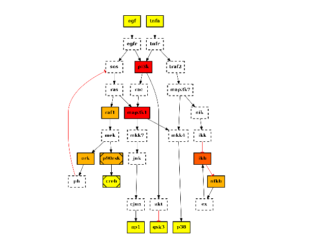
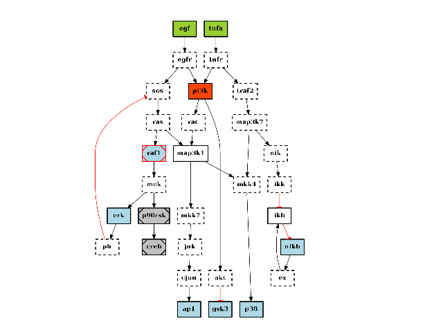
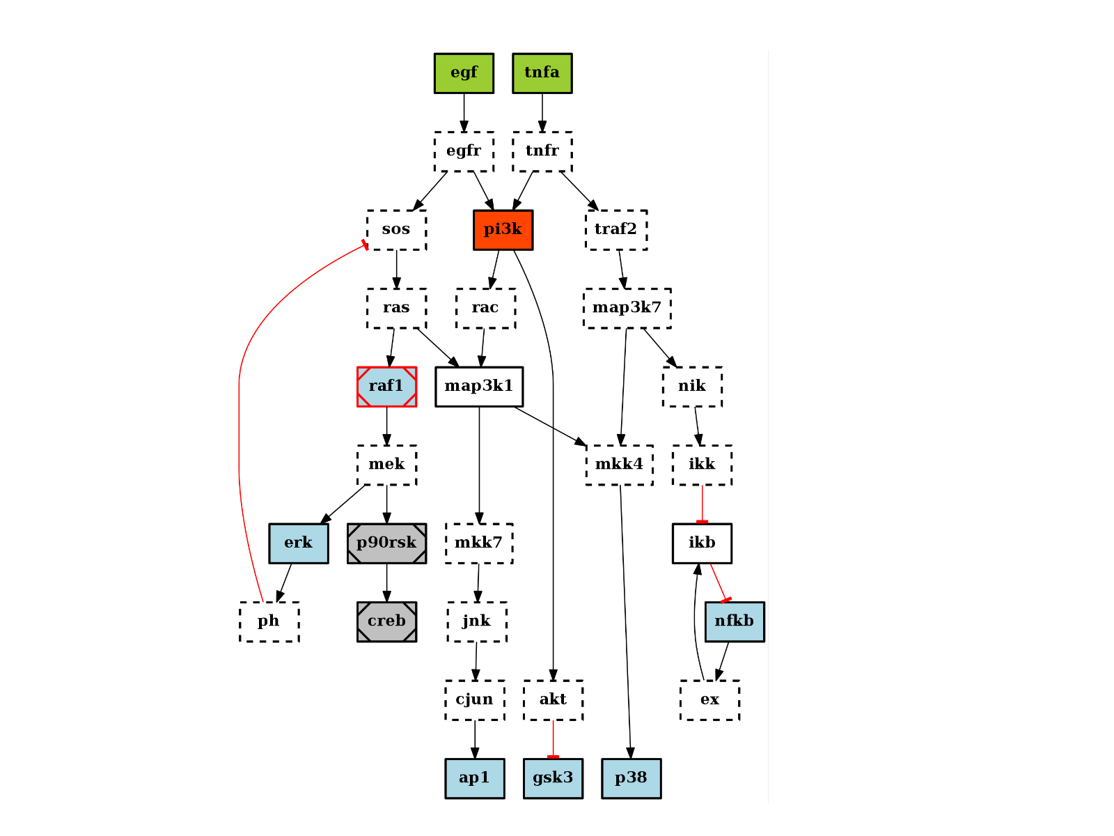
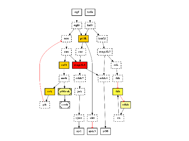
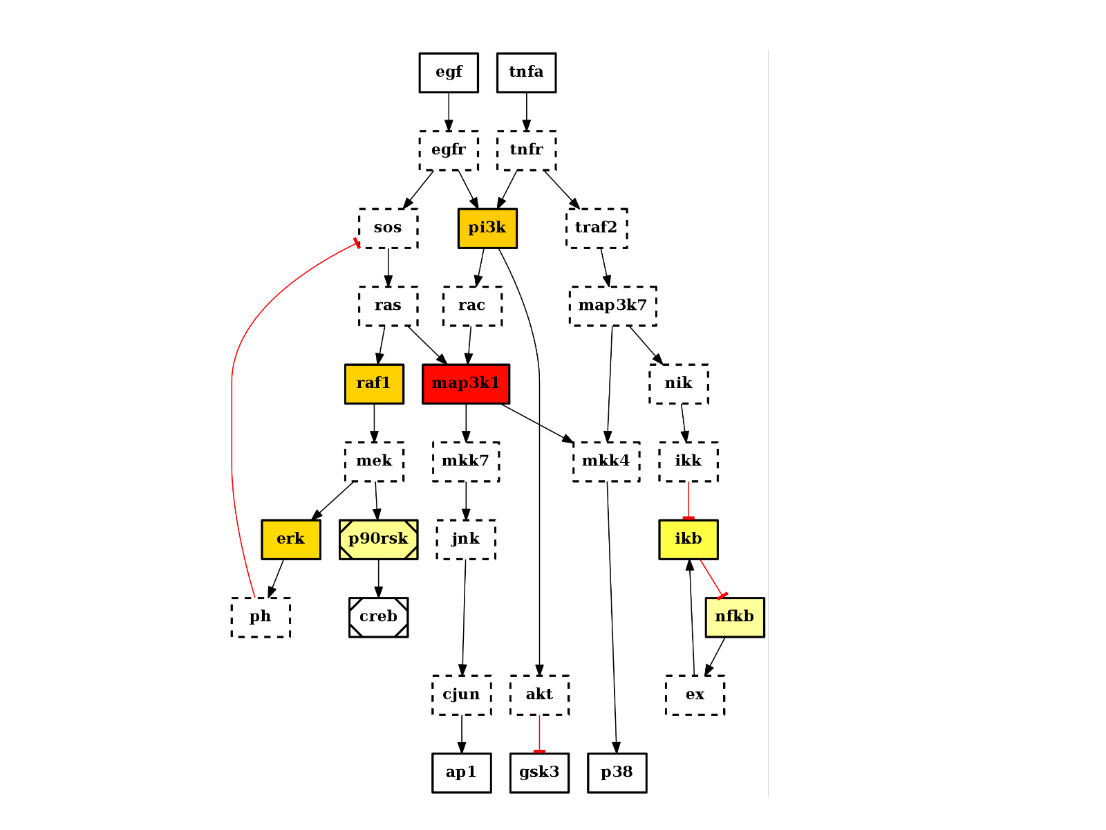
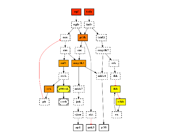
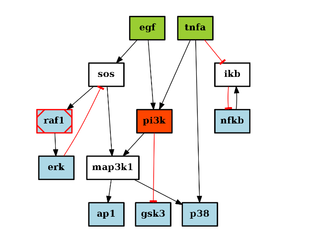
There are plotting functionalities to look at the graph, which are based on graphviz library. For instance, the plot() function is quite flexible. If a MIDAS file is provided, the default behaviour follow CellNOptR convention, where stimuli are colored in green, inhibitors in red and measurements in blue:
from cno import CNOGraph, cnodata
pknmodel = cnodata("PKN-ToyPB.sif")
data = cnodata("MD-ToyPB.csv")
c = CNOGraph(pknmodel, data)
c.plot()
(Source code, png, hires.png, pdf)

If you did not use any MIDAS file as input parameter, you can still populate the hidden fields _stimuli, _inhibitors, _signals.
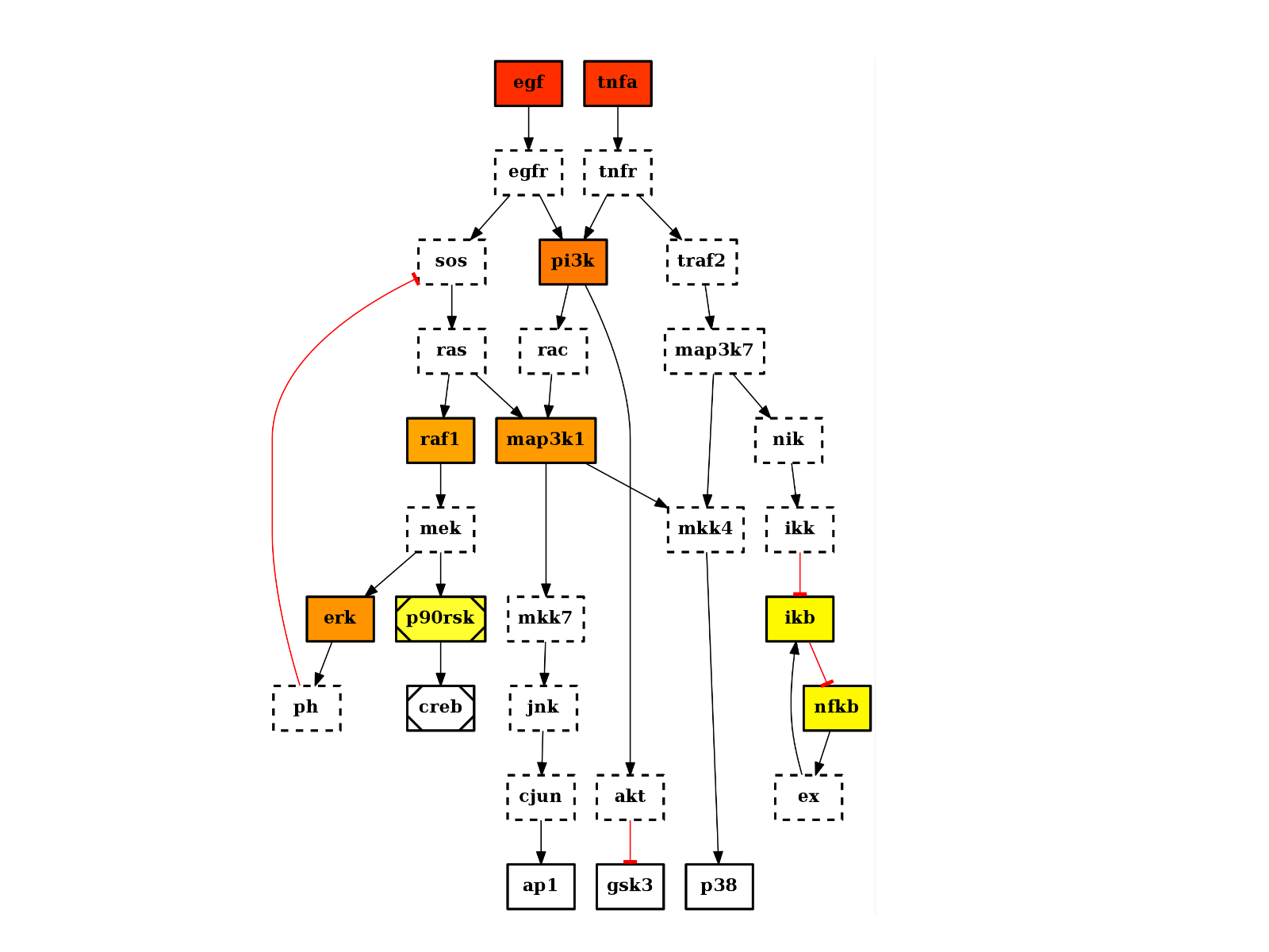
You can also overwrite this behaviour by using the node_attribute parameter when calling plot(). For instance, if you call centrality_degree(), which computes and populate the node attribute degree. You can then call plot as follows to replace the default color:
from cno import CNOGraph, cnodata
pknmodel = cnodata("PKN-ToyPB.sif")
data = cnodata("MD-ToyPB.csv")
c = CNOGraph(pknmodel, data)
c.centrality_degree()
c.plot(node_attribute="centrality_degree", colorbar)
Similarly, you can tune the color of the edge attribute. See the plot() for more details.
See also
tutorial, user guide
See also
The cno.io.xcnograph.XCNOGraph provides many more tools for plotting various information on the graph structure.
Constructor
Parameters: - add_cycle(nodes, **attr)[source]
Add a cycle
Parameters: - nodes (list) – a list of nodes. A cycle will be constructed from the nodes (in order) and added to the graph.
- attr (dict) – must provide the “link” keyword. Valid values are “+”, “-” the links of every edge in the cycle will be identical.
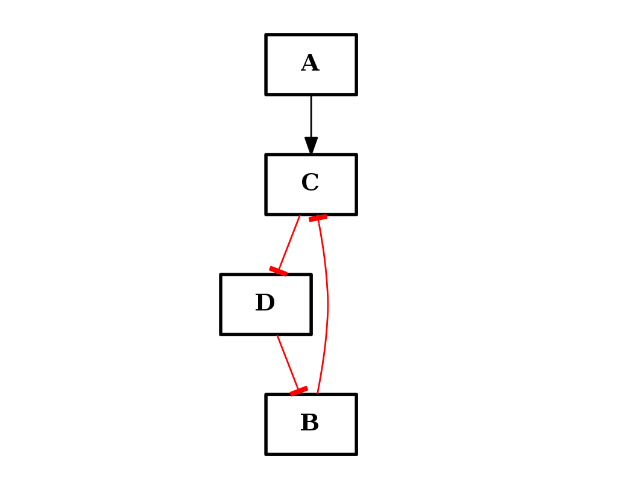
from cno import CNOGraph
c = CNOGraph()
c.add_edge("A", "C", link="+")
c.add_edge("B", "C", link="+")
c.add_cycle(["B", "C", "D"], link="-")
c.plot()
(Source code, png, hires.png, pdf)

Warning
added cycle overwrite previous edges
- add_edge(u, v, attr_dict=None, **attr)[source]
adds an edge between node u and v.
Parameters: - u (str) – source node
- v (str) – target node
- link (str) – compulsary keyword. must be “+” or “-“
- attr_dict (dict) – dictionary, optional (default= no attributes) Dictionary of edge attributes. Key/value pairs will update existing data associated with the edge.
- attr – keyword arguments, optional edge data (or labels or objects) can be assigned using keyword arguments. keywords provided will overwrite keys provided in the attr_dict parameter
Warning
color, penwidth, arrowhead keywords are populated according to the value of the link.
- If link=”+”, then edge is black and arrowhead is normal.
- If link=”-”, then edge is red and arrowhead is a tee
from cno import CNOGraph
c = CNOGraph()
c.add_edge("A","B",link="+")
c.add_edge("A","C",link="-")
c.add_edge("C","D",link="+", mycolor="blue")
c.add_edge("C","E",link="+", data=[1,2,3])
If you want multiple edges, use add_reaction() method.
c.add_reaction(“A+B+C=D”)equivalent to
c.add_edge("A", "D", link="+")
c.add_edge("B", "D", link="+")
c.add_edge("C", "D", link="+")
Attributes on the edges can be provided using the parameters attr_dict (a dictionary) and/or **attr, which is a list of key/value pairs. The latter will overwrite the key/value pairs contained in the dictionary. Consider this example:
c = CNOGraph()
c.add_edge("a", "c", attr_dict={"k":1, "data":[0,1,2]}, link="+", k=3)
c.edges(data=True)
[('a',
'c',
    {'arrowhead': 'normal',
    'color': 'black',
    'compressed': [],
    'k':3
    'link': '+',
    'penwidth': 1})]
The field “k” in the dictionary (attr_dict) is set to 1. However, it is also provided as an argument but with the value 3. The latter is the one used to populate the edge attributes, which can be checked by printing the data of the edge (c.edges(data=True())
See also
special attributes are automatically set by get_default_edge_attributes(). the color of the edge is black if link is set to “+” and red otherwie.
- add_node(node, attr_dict=None, **attr)[source]
Add a node
Parameters: - node (str) – a node to add
- attr_dict (dict) – dictionary, if None, replace by default shape/color. recognised keys are those from graphviz. Default keys set are color, fillcolor, shape, style, penwidth
- attr – additional keyword provided will overwrite keys found in attr_dict parameter
c = CNOGraph()
c.add_node("A", data=[1,2,3,])
c.add_node("B", shape='circle')
Warning
attr replaces any key found in attr_dict. See add_edge() for details.
Todo
currently nodes that contains a ^ sign are interpreted as AND gate and will appear as small circle. One way to go around is to use the label attribute. you first add the node with a differnt name and populate the label with the correct nale (the one that contain the ^ sign); When calling the plot function, they should all appear as expected.
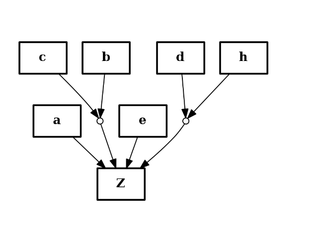
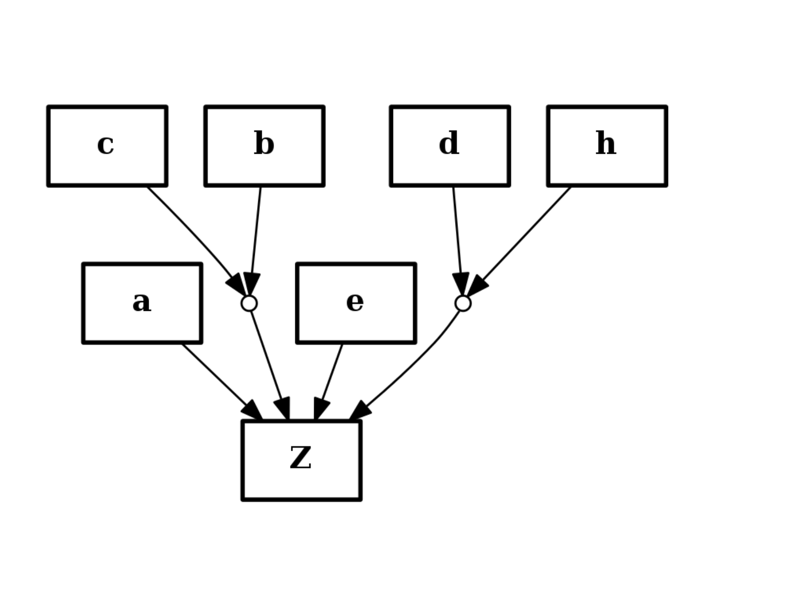
- add_reaction(*args, **kargs)[source]
Add nodes and edges given a reaction
Parameters: reac (str) – a valid reaction. See below for examples Here are some valid reactions that includes NOT, AND and OR gates. + is an OR and ^ character is an AND gate:
>>> s.add_reaction("A=B")
>>> s.add_reaction("A+B=C")
>>> s.add_reaction("A^C=E")
>>> s.add_reaction("!F+G=H")
from cno import CNOGraph
c = CNOGraph()
c.add_reaction("a+b^c+e+d^h=Z")
c.plot()
(Source code, png, hires.png, pdf)

Warning
component of AND gates are ordered alphabetically.
- adjacency_matrix(nodelist=None, weight=None)[source]
Return adjacency matrix.
Parameters: - nodelist (list) – The rows and columns are ordered according to the nodes in nodelist. If nodelist is None, then the ordering is produced by nodes() method.
- weight (str) – (default=None) The edge data key used to provide each value in the matrix. If None, then each edge has weight 1. Otherwise, you can set it to “weight”
Returns: numpy matrix Adjacency matrix representation of CNOGraph.
Note
alias to networkx.adjacency_matrix()
See also
adjacency_iter() and adjacency_list()
- attributes = None
nodes and edges attributes. See CNOGraphAttributes
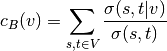
- centrality_betweeness(k=None, normalized=True, weight=None, endpoints=False, seed=None)[source]
Compute the shortest-path betweeness centrality for nodes.
Betweenness centrality of a node v is the sum of the fraction of all-pairs shortest paths that pass through v:
where
 is the set of nodes,
  is the number of
shortest
is the number of
shortest  -paths, and
  is the number of those
paths passing through some node
is the number of those
paths passing through some node  other than
  .
If
.
If  ,
,  , and if
  ,
,
 .
.Parameters: - k (int) – (default=None) If k is not None use k node samples to estimate betweeness. The value of k <= n where n is the number of nodes in the graph. Higher values give better approximation.
- normalized (bool) – If True the betweeness values are normalized by
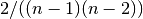 for graphs, and
 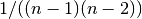 for directed graphs where
  is the number of nodes in G.
 - weight (str) – None or string, optional If None, all edge weights are considered equal.
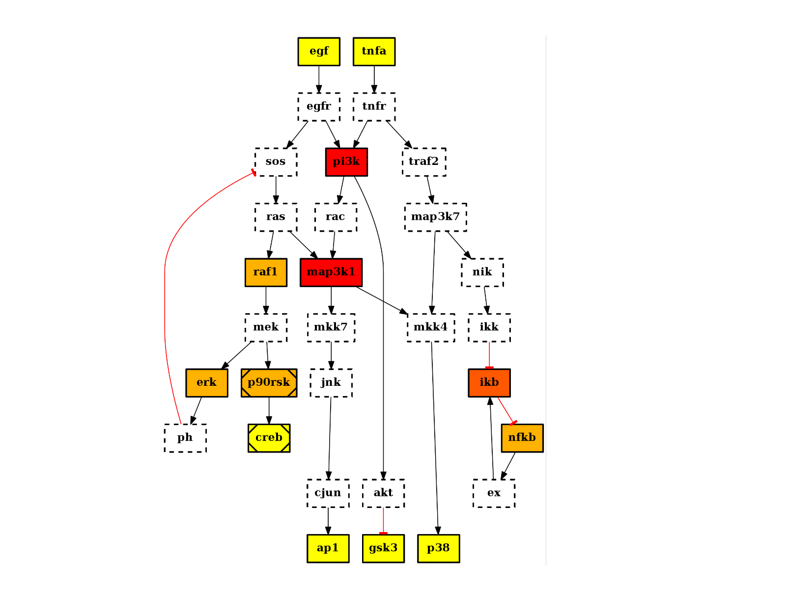
from cno import CNOGraph, cnodata
c = CNOGraph(cnodata("PKN-ToyPB.sif"), cnodata("MD-ToyPB.csv"))
c.centrality_betweeness()
c.plot(node_attribute="centrality_betweeness")
(Source code, png, hires.png, pdf)

See also
networkx.centrality.centrality_betweeness
- centrality_closeness(**kargs)[source]
Compute closeness centrality for nodes.
Closeness centrality at a node is 1/average distance to all other nodes.
Parameters: - v – node, optional Return only the value for node v
- distance (str) – string key, optional (default=None) Use specified edge key as edge distance. If True, use ‘weight’ as the edge key.
- normalized (bool) – optional If True (default) normalize by the graph size.
Returns: Dictionary of nodes with closeness centrality as the value.
from cno import CNOGraph, cnodata
c = CNOGraph(cnodata("PKN-ToyPB.sif"), cnodata("MD-ToyPB.csv"))
c.centrality_closeness()
c.plot(node_attribute="centrality_closeness")
(Source code, png, hires.png, pdf)

- centrality_degree()[source]
Compute the degree centrality for nodes.
The degree centrality for a node v is the fraction of nodes it is connected to.
Returns: list of nodes with their degree centrality. It is also added to the list of attributes with the name “degree_centr” from cno import CNOGraph, cnodata c = CNOGraph(cnodata("PKN-ToyPB.sif"), cnodata("MD-ToyPB.csv")) c.centrality_degree() c.plot(node_attribute="centrality_degree")
(Source code, png, hires.png, pdf)
- check_data_compatibility()[source]
When setting a MIDAS file, need to check that it is compatible with the graph, i.e. species are found in the model.
- clean_orphan_ands(*args, **kargs)[source]
Remove AND gates that are not AND gates anymore
When removing an edge or a node, AND gates may not be valid anymore either because the output does not exists or there is a single input.
This function is called when remove_node() or remove_edge() are called. However, if you manipulate the nodes/edges manually you may need to call this function afterwards.
- collapse_node(node)[source]
Collapses a node (removes a node but connects input nodes to output nodes)
This is different from remove_node(), which removes a node and its edges thus creating non-connected graph. collapse_node(), instead remove the node but merge the input/output edges IF possible. If there are multiple inputs AND multiple outputs the node is not removed.
Parameters: node (str) – a node to collapse. - Nodes are collapsed if there is at least one input or output.
- Node are not removed if there is several inputs and several ouputs.
- if the input edge is -, and the next is + or viceversa then the final edge if -
- if the input edge is - and output is - then final edge is +
- compress(recursive=True, iteration=1, max_iteration=5)[source]
Finds compressable nodes and removes them from the graph
A compressable node is a node that is not part of the special nodes (stimuli/inhibitors/readouts mentionned in the MIDAS file). Nodes that have multiple inputs and multiple outputs are not compressable either.
from cno import CNOGraph, cnodata
c = CNOGraph(cnodata("PKN-ToyPB.sif"), cnodata("MD-ToyPB.csv"))
c.cutnonc()
c.compress()
c.plot()
(Source code, png, hires.png, pdf)

See also
- compressable_nodes
Returns list of compressable nodes (Read-only).
- cutnonc()[source]
Finds non-observable and non-controllable nodes and removes them.
from cno import CNOGraph, cnodata
c = CNOGraph(cnodata("PKN-ToyPB.sif"), cnodata("MD-ToyPB.csv"))
c.cutnonc()
c.plot()
(Source code, png, hires.png, pdf)
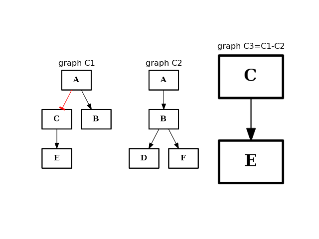
- difference(other)[source]
Return a CNOGraph instance that is the difference with the input graph
(i.e. all elements that are in this set but not the others.)
from cno import CNOGraph
from pylab import subplot, title

c1 = CNOGraph()
c1.add_edge("A", "B", link="+")
c1.add_edge("A", "C", link="-")
c1.add_edge("C", "E", link="+")
subplot(1,3,1)
title("graph C1")
c1.plot(hold=True)

c2 = CNOGraph()
c2.add_edge("A", "B", link="+")
c2.add_edge("B", "D", link="+")
c2.add_edge("B", "F", link="+")
subplot(1,3,2)
c2.plot(hold=True)
title("graph C2")

c3 = c1.difference(c2)
subplot(1,3,3)
c3.plot(hold=True)
title("graph C3=C1-C2")
(Source code, png, hires.png, pdf)

Note
this method should be equivalent to the - operator. So c1-c2 == c1.difference(c2)
- draw(prog='dot', attribute='fillcolor', hold=False, **kargs)[source]
Draw the network using matplotlib. Not exactly what we want but could be useful.
Parameters: - prog (str) – one of the graphviz program (default dot)
- hold (bool) – hold previous plot (default is False)
- attribute (str) – attribute to use to color the nodes (default is “fillcolor”).
- node_size – default 1200
- width – default 2
Uses the fillcolor attribute of the nodes Uses the link attribute of the edges
See also
plot() that is dedicated to this kind of plot using graphviz
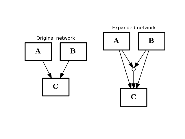
- expand_and_gates(maxInputsPerGate=2)[source]
Expands the network to incorporate AND gates
Parameters: maxInputsPerGate (int) – restrict maximum number of inputs used to create AND gates (default is 2) The CNOGraph instance can be used to model a boolean network. If a node has several inputs, then the combinaison of the inputs behaves like an OR gate that is we can take the minimum over the inputs.
In order to include AND behaviour, we introduce a special node called AND gate. This function adds AND gates whenever a node has several inputs. The AND gates can later on be used in a boolean formalism.
In order to recognise AND gates, we name them according to the following rule. If a node A has two inputs B and C, then the AND gate is named:
B^C=A
and 3 edges are added: B to the AND gates, C to the AND gates and the AND gate to A.
If an edge is a “-” link then, an ! character is introduced.
In this expansion process, AND gates themselves are ignored.
If there are more than 2 inputs, all combinaison of inputs may be considered but the default parameter maxInputsPerGate is set to 2. For instance, with 3 inputs A,B,C you may have the following combinaison: A^B, A^C, B^C. The link A^B^C will be added only if maxInputsPerGate is set to 3.
from cno import CNOGraph
from pylab import subplot, title

c = CNOGraph()
c.add_edge("A", "C", link="+")
c.add_edge("B", "C", link="+")
subplot(1,2,1)
title("Original network")
c.plot(hold=True)

c.expand_and_gates()
subplot(1,2,2)
c.plot(hold=True)
title("Expanded network")
(Source code, png, hires.png, pdf)

See also
Note
this method adds all AND gates in one go. If you want to add a specific AND gate, you have to do it manually. You can use the add_reaction() for that purpose.
Note
propagate data from edge on the AND gates.
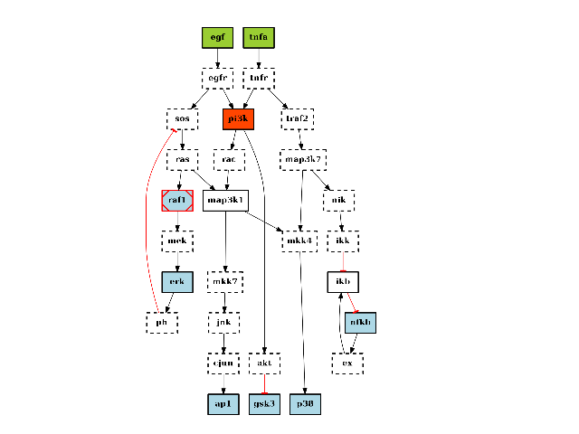
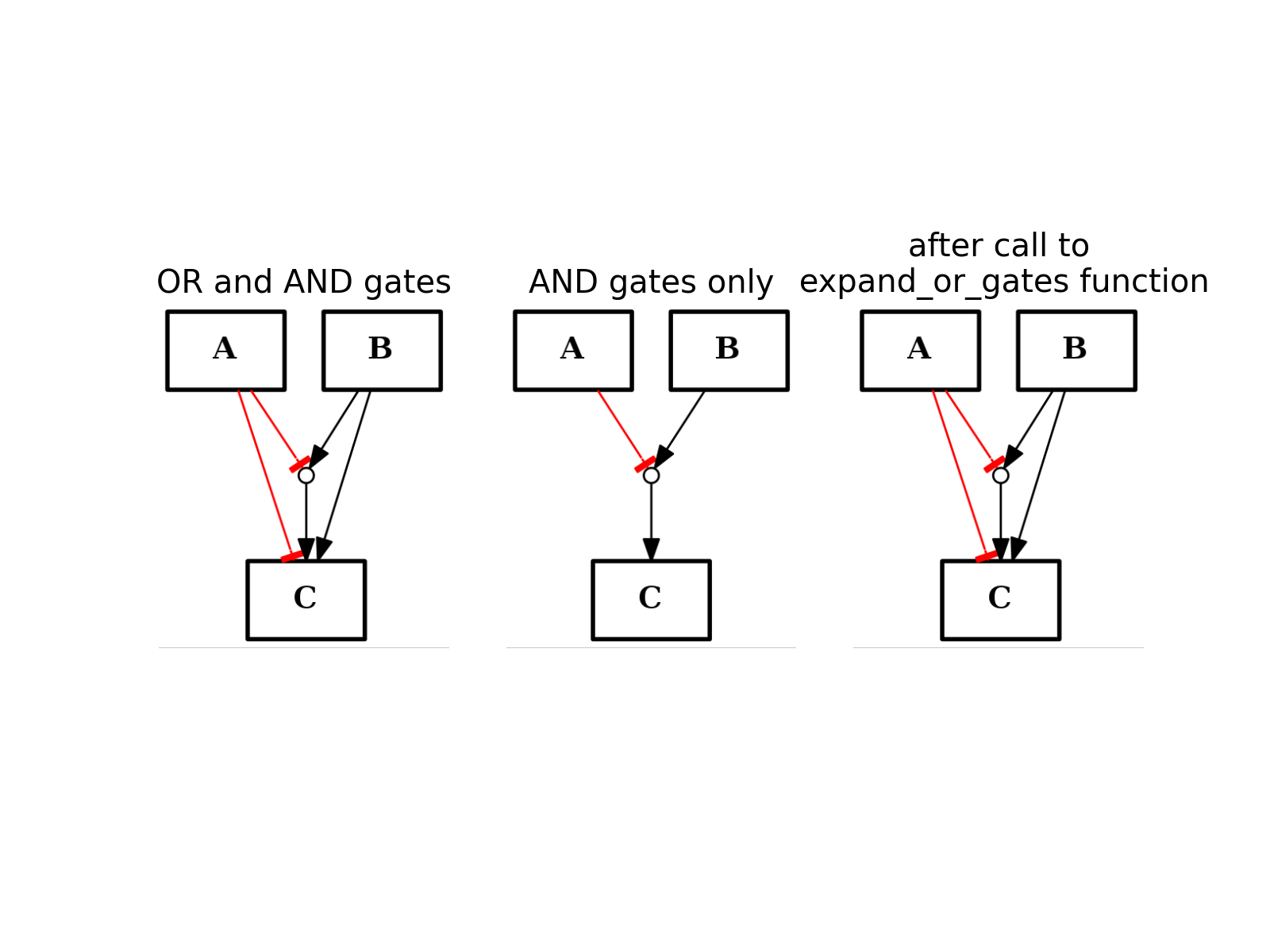
- expand_or_gates()[source]
Expand OR gates given AND gates
If a graph contains AND gates (without its OR gates), you can add back the OR gates automatically using this function.
from cno import CNOGraph
from pylab import subplot, title

c1 = CNOGraph()
c1.add_edge("A", "C", link="-")
c1.add_edge("B", "C", link="+")
c1.expand_and_gates()
subplot(1,3,1)
title("OR and AND gates")
c1.plot(hold=True)

c1.remove_edge("A", "C")
c1.remove_edge("B", "C")
subplot(1,3,2)
c1.plot(hold=True)
title("AND gates only")

c1.expand_or_gates()
subplot(1,3,3)
c1.plot(hold=True)
title("after call to \n expand_or_gates function")
(Source code, png, hires.png, pdf)
See also
- findnonc()[source]
Finds the Non-Observable and Non-Controllable nodes
- Non observable nodes are those that do not have a path to any measured species in the PKN
- Non controllable nodes are those that do not receive any information from a species that is perturbed in the data.
Such nodes can be removed without affecting the readouts.
Parameters: - G – a CNOGraph object
- stimuli – list of stimuli
- stimuli – list of signals
Returns: a list of names found in G that are NONC nodes
>>> from cno import CNOGraph, cnodata
>>> model = cnodata('PKN-ToyMMB.sif')
>>> data = cnodata('MD-ToyMMB.csv')
>>> c = CNOGraph(model, data)
>>> namesNONC = c.nonc()
Details: Using a floyd Warshall algorithm to compute path between nodes in a directed graph, this class identifies the nodes that are not connected to any signals (Non Observable) and/or any stimuli (Non Controllable) excluding the signals and stimuli, which are kept whatever is the outcome of the FW algorithm.
- get_max_rank()[source]
Get the maximum rank from the inputs using floyd warshall algorithm
If a MIDAS file is provided, the inputs correspond to the stimuli. Otherwise, (or if there is no stimuli in the MIDAS file), use the nodes that have no predecessors as inputs (ie, rank=0).
- get_node_attributes(node)[source]
Returns attributes of a node using the MIDAS attribute
Given a node, this function identifies the type of the input node and returns a dictionary with the relevant attributes found in node_attributes.attributes.
For instance, if a midas file exists and if node belongs to the stimuli, then the dicitonary returned contains the color green.
Parameters: node (str) – Returns: dictionary of attributes.
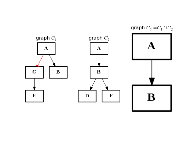
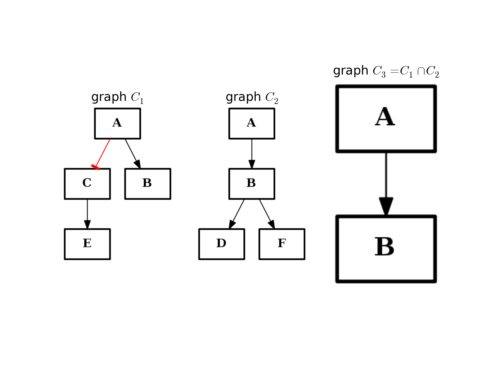
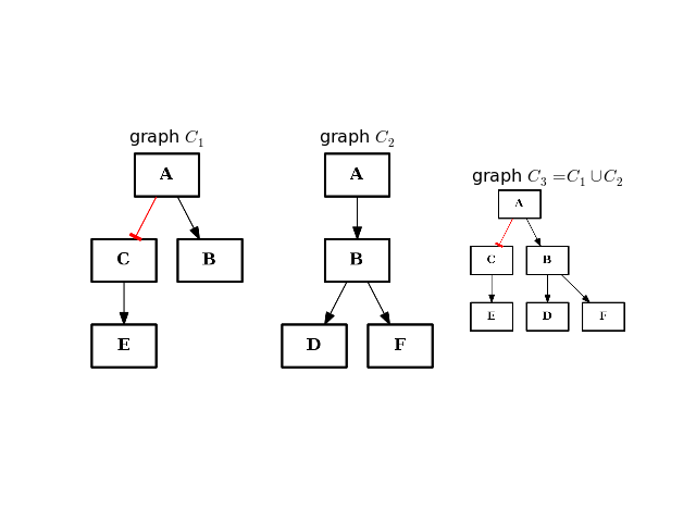
- intersect(other)[source]
Return a graph with only nodes found in “other” graph.
from cno import CNOGraph
from pylab import subplot, title

c1 = CNOGraph()
c1.add_edge("A", "B", link="+")
c1.add_edge("A", "C", link="-")
c1.add_edge("C", "E", link="+")
subplot(1,3,1)
title(r"graph $C_1$")
c1.plot(hold=True)

c2 = CNOGraph()
c2.add_edge("A", "B", link="+")
c2.add_edge("B", "D", link="+")
c2.add_edge("B", "F", link="+")
subplot(1,3,2)
c2.plot(hold=True)
title(r"graph $C_2$")

c3 = c1.intersect(c2)
subplot(1,3,3)
c3.plot(hold=True)
title(r"graph $C_3 = C_1 \cap C_2$")
(Source code, png, hires.png, pdf)

- is_compressable(node)[source]
Returns True if the node can be compressed, False otherwise
Parameters: node (str) – a valid node name Returns: boolean value Here are the rules for compression. The main idea is that a node can be removed if the boolean logic is preserved (i.e. truth table on remaining nodes is preserved).
A node is compressable if it is not part of the stimuli, inhibitors, or signals specified in the MIDAS file.
If a node has several outputs and inputs, it cannot be compressed.
If a node has one input or one output, it may be compressed. However, we must check the following possible ambiguity that could be raised by the removal of the node: once removed, the output of the node may have multiple input edges with different types of inputs edges that has a truth table different from the original truth table. In such case, the node cannot be compressed.
Finally, a node cannot be compressed if one input is also an output (e.g., cycle).
from cno import CNOGraph
from pylab import subplot,show, title
c = cnograph.CNOGraph()
c.add_edge("a", "c", link="-")
c.add_edge("b", "c", link="+")
c.add_edge("c", "d", link="+")
c.add_edge("b", "d", link="-")
c.add_edge("d", "e", link="-")
c.add_edge("e", "g", link="+")
c.add_edge("g", "h", link="+")
c.add_edge("h", "g", link="+")

# multiple inputs/outputs are not removed
c.add_edge("s1", "n1", link="+")
c.add_edge("s2", "n1", link="+")
c.add_edge("n1", "o1", link="+")
c.add_edge("n1", "o2", link="+")

c._stimuli = ["a", "b", "s1", "s2"]
c._signals = ["d", "g", "o1", "o2"]

subplot(1,2,1)
c.plot(hold=True)
title("Initial graph")

c.compress()
subplot(1,2,2)
c.plot(hold=True)
title("compressed graph")

show()
- is_reaction_in(reaction)[source]
Return boolean with present of a reaction in the network
Parameters: reaction – a valid reaction Todo
Could be a string of reaction
- lookfor(specyName)[source]
Prints information about a species
If not found, try to find species by ignoring cases.
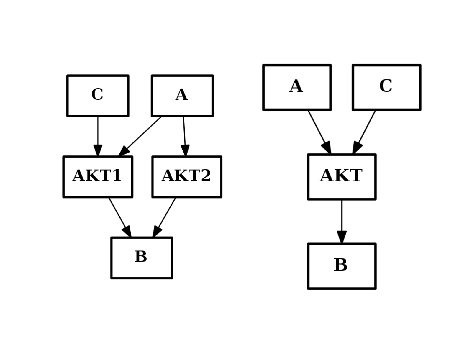
- merge_nodes(nodes, node)[source]
Merge several nodes into a single one
from cno import CNOGraph
from pylab import subplot
c = CNOGraph()
c.add_edge("AKT2", "B", link="+")
c.add_edge("AKT1", "B", link="+")
c.add_edge("A", "AKT2", link="+")
c.add_edge("A", "AKT1", link="+")
c.add_edge("C", "AKT1", link="+")
subplot(1,2,1)
c.plot(hold=True)
c.merge_nodes(["AKT1", "AKT2"], "AKT")
subplot(1,2,2)
c.plot(hold=True)
(Source code, png, hires.png, pdf)

- midas
MIDAS Read/Write attribute.
- nonc
Returns list of Non observable and non controlable nodes (Read-only).
- plot(prog='dot', viewer='pylab', hold=False, show=True, filename=None, node_attribute=None, edge_attribute=None, cmap='heat', colorbar=False, remove_dot=True, normalise_cmap=True, edge_attribute_labels=True, rank_method='inout')[source]
plotting graph using dot program (graphviz) and networkx
By default, a temporary file is created to hold the image created by graphviz, which is them shown using pylab. You can choose not to see the image (show=False) and to save it in a local file instead (set the filename). The output format is PNG. You can play with networkx.write_dot to save the dot and create the SVG yourself.
Parameters: - prog (str) – the graphviz layout algorithm (default is dot)
- viewer – pylab
- show (bool) – show the plot (True by default)
- remove_dot (bool) – if True, remove the temporary dot file.
- edge_attribute_labels – is True, if the label are available, show them. otherwise, if edge_attribute is provided, set lael as the edge_attribute
- rank_method – If none, let graphviz do the job. Issue is that (i) input stimuli may not be aligned and output neither. The rank_method set to cno constraints the stimuli and measured species that are sinks all others are free. The same constraint all nodes with same rank to be in the same subgraph.
Additional attributes on the graph itself can be set up by populating the graph attribute with a dictionary called “graph”:
c.graph['graph'] = {"splines":True, "size":(20,20), "dpi":200}
Useful other options are:
c.edge["tnfa"]["tnfr"]["penwidth"] = 3
c.edge["tnfa"]["tnfr"]["label"] = " 5"
If you use edge_attribute and show_edge_labels, label are replaced by the content of edge_attribute. If you still want differnt labels, you must stet show_label_edge to False and set the label attribute manually
c = cnograph.CNOGraph()
c.add_reaction("A=C")
c.add_reaction("B=C")
c.edge['A']['C']['measure'] = 0.5
c.edge['B']['C']['measure'] = 0.1
c.expand_and_gates()
c.edge['A']['C']['label'] = "0.5 seconds"
# compare this that shows only one user-defined label
c.plot()
# with that show all labels
c.plot(edge_attribute="whatever", edge_attribute_labels=False)
See the graphviz homepage documentation for more options.
c.plot(filename='test.svg', viewer='yout_favorite_viewer',
    remove_dot=False, rank_method='cno')
Note
edge attribute in CNOGraph (Directed Graph) are not coded in the same way in CNOGraphMultiEdges (Multi Directed Graph). So, this function does not work for MultiGraph
Todo
use same colorbar as in midas. rigtht now; the vmax is not correct.
Todo
precision on edge_attribute to 2 digits.
if filename provided with extension different from png, pylab must be able to read the image. If not, you should set viewer to something else.
c.plot() # uses default layout, with PNG format viewed with pylab c.plot(rank_method=’same’) # uses ranks of each node with PNG format viewed with pylab c.plot(rank_method=’cno’, filename=’test.svg’, viewer=’browse’) # uses browse (defautl viewer) c.plot(rank_method=’cno’, filename=’test.svg’, viewer=’browse’)
- preprocessing(expansion=True, compression=True, cutnonc=True, maxInputsPerGate=2)[source]
Performs the 3 preprocessing steps (cutnonc, expansion, compression)
Parameters: - expansion (bool) – calls expand_and_gates() method
- compression (bool) – calls compress() method
- cutnon (bool) – calls cutnonc() method
- maxInputPerGates (int) – parameter for the expansion step
from cno import CNOGraph, cnodata
c = CNOGraph(cnodata("PKN-ToyPB.sif"), cnodata("MD-ToyPB.csv"))
c.preprocessing()
c.plot()
(Source code, png, hires.png, pdf)

- reactions
return the reactions (edges)
- read_json(filename)[source]
Load a network in JSON format as exported from to_json()
Parameters: filename (str) – See also
- relabel_nodes(mapping, inplace=True)[source]
Function to rename a node, while keeping all its attributes.
Parameters: mapping (dict) – a dictionary mapping old names (keys) to new names (values ) Returns: new CNOGraph object if we take this example:
c = CNOGraph();
c.add_reaction("a=b");
c.add_reaction("a=c");
c.add_reaction("b=d");
c.add_reaction("c=d");
c.expand_and_gates()
Here, an AND gate has been created. c.nodes() tells us that its name is “b^c=d”. If we rename the node b to blong, the AND gate name is unchanged if we use the nx.relabel_nodes function. Visually, it is correct but internally, the “b^c=d” has no more meaning since the node “b” does not exist anymore. This may lead to further issues if we for instance split the node c:
c = nx.relabel_nodes(c, {"b": "blong"})
c.split_node("c", ["c1", "c2"])
This function calls relabel_node taking care of the AND nodes as well.
Warning
inplace modifications
Todo
midas must also be modified
- remove_and_gates(*args, **kargs)[source]
Remove the AND nodes added by expand_and_gates()
- remove_edge(u, v)[source]
Remove the edge between u and v.
Parameters: - u (str) – node u
- u – node v
Calls clean_orphan_ands() afterwards
- remove_node(*args, **kargs)[source]
Remove a node n
Parameters: node (str) – the node to be removed Edges linked to n are also removed. AND gate may now be irrelevant (only one input or no input) and are therefore removed as well.
See also
- remove_nodes_from(nbunch)[source]
Removes a bunch of nodes
Warning
need to be tests with and gates.
- reset_edge_attributes()[source]
set all edge attributes to default attributes
See also
get_default_edge_attribute()
if we set an edge label, which is an AND ^, then plot fails in this function c.edge[“alpha^NaCl=HOG1”][‘label’] = ”?”
- set_node_attributes(attr_dict)[source]
Experimental
dictionaries where keys are nodes and keys are dictionaries of attributes. Does not need to be
{‘Akt’: {‘color’:red’, ‘strength’:0.5}} Does not need to have a value for each node could set default values may be ?
- species
Return sorted list of species (ignoring and gates) Read-only attribute.
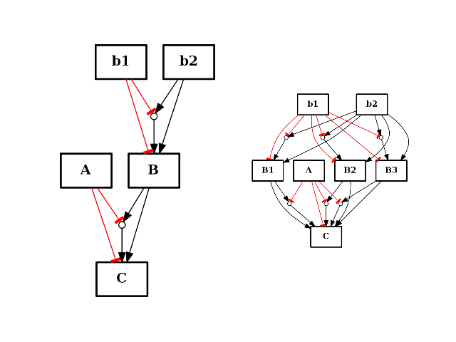
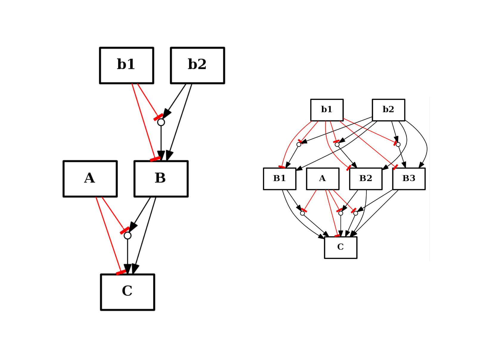
- split_node(node, nodes)[source]
from cno import CNOGraph
from pylab import subplot
c = CNOGraph()
c.add_reaction("!A=C")
c.add_reaction("B=C")
c.add_reaction("!b1=B")
c.add_reaction("b2=B")
c.expand_and_gates()

subplot(1,2,1)
c.plot(hold=True)

c.split_node("B", ["B1", "B2", "B3"])
subplot(1,2,2)
c.plot(hold=True)
(Source code, png, hires.png, pdf)

- swap_edges(nswap=1, inplace=True, self_loop=False)[source]
Swap two edges in the graph while keeping the node degrees fixed.
A double-edge swap two randomly chosen edges u-v and x-y and creates the new edges u-x and v-y:
u  v                u  v
|  |     becomes    |  |
x  y                y  x
If either the edge u-x or v-y already exist no swap is performed and another attempt is made to find a suitable edge pair.
Parameters: nswap (int) – number of swaps to perform (Defaults to 1) Returns: nothing Warning
the graph is modified in place.
Warning
and gates are removed at the beginning since they do not make sense with the new topolgy. They can easily be added back
a proposal swap is ignored in 3 cases: #. if the summation of in_degree is changed #. if the summation of out_degree is changed #. if resulting graph is disconnected
Note
what about self loop ? if proposed, there are ignored except if required to be kept
- to_gexf(filename)[source]
Export into GEXF format
Parameters: filename (str) – This is the networkx implementation and requires the version 1.7 This format is quite rich and can be used in external software such as Gephi.
Warning
color and labels are lost. information is stored as attributes.and should be as properties somehow. Examples: c.node[‘mkk7’][‘viz’] = {‘color’: {‘a’: 0.6, ‘r’: 239, ‘b’: 66,’g’: 173}}
- to_json(filename=None)[source]
Export the graph into a JSON format
Parameters: filename (str) – See also
loadjson()
- to_sbmlqual(filename=None)[source]
Export the topology into SBMLqual and save in a file
Parameters: filename (str) – if not provided, returns the SBML as a string. Returns: nothing if filename is not provided See also
cno.io.sbmlqual()
- to_sif(filename=None)[source]
Export CNOGraph into a SIF file.
Takes into account and gates. If a species called “A^B=C” is found, it is an AND gate that is encoded in a CSV file as:
A 1 and1
B 1 and1
and1 1 C
Parameters: filename (str) –
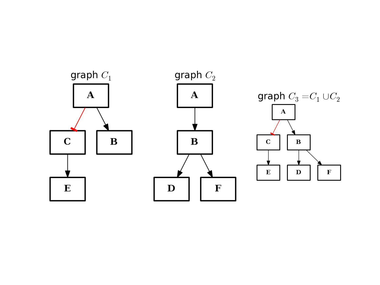
- union(other)[source]
Return graph with elements from this instance and the input graph.
from cno import CNOGraph
from pylab import subplot, title

c1 = CNOGraph()
c1.add_edge("A", "B", link="+")
c1.add_edge("A", "C", link="-")
c1.add_edge("C", "E", link="+")
subplot(1,3,1)
title(r"graph $C_1$")
c1.plot(hold=True)

c2 = CNOGraph()
c2.add_edge("A", "B", link="+")
c2.add_edge("B", "D", link="+")
c2.add_edge("B", "F", link="+")
subplot(1,3,2)
c2.plot(hold=True)
title(r"graph $C_2$")

c3 = c1.union(c2)
subplot(1,3,3)
c3.plot(hold=True)
title(r"graph $C_3 = C_1 \cup C_2$")
(Source code, png, hires.png, pdf)

- verbose
1.1.2. XCNOGraph
- class XCNOGraph(model=None, midas=None, verbose=False)[source]
Extra plotting and statistical tools related to CNOGraph
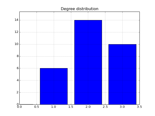
- degree_histogram(show=True, normed=False)[source]
Compute histogram of the node degree (and plots the histogram)
from cno import XCNOGraph, cnodata
c = XCNOGraph(cnodata("PKN-ToyPB.sif"), cnodata("MD-ToyPB.csv"))
c.degree_histogram()
(Source code, png, hires.png, pdf)

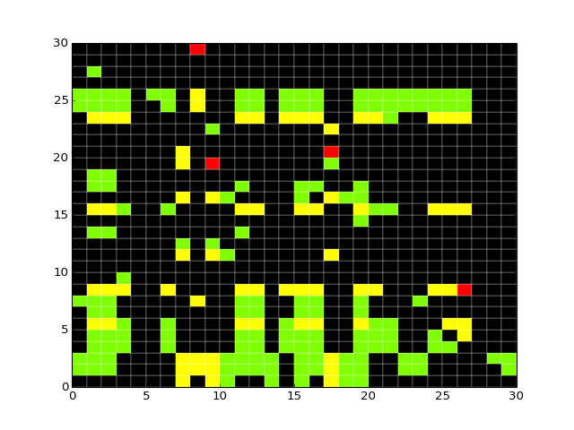
- dependency_matrix(fontsize=12)[source]
Return dependency matrix
 = green ; species i is an activator of species j (only positive path)
- = red ; species i is an inhibitor of species j (only negative path)
- = yellow; ambivalent (positive and negative paths connecting i and j)
- = red ; species i has no influence on j
from cno import XCNOGraph, cnodata
c = XCNOGraph(cnodata("PKN-ToyPB.sif"), cnodata("MD-ToyPB.csv"))
c.dependency_matrix()
(Source code, png, hires.png, pdf)

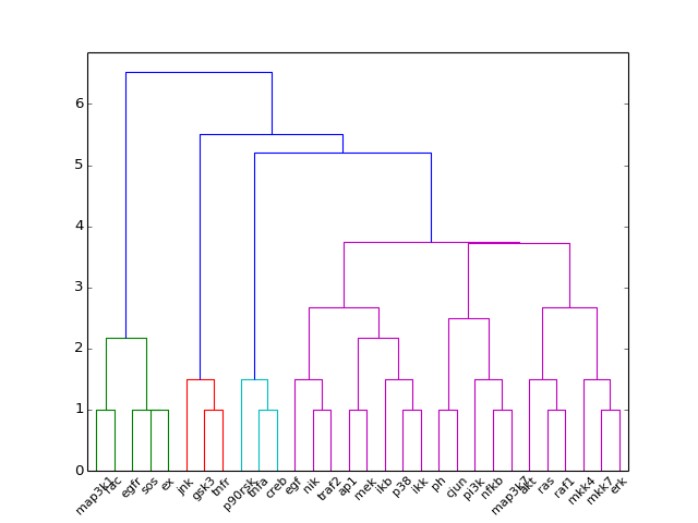
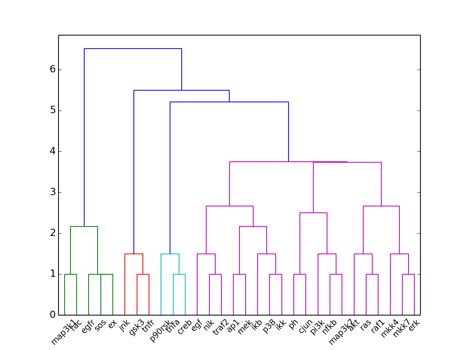
- hcluster()[source]
from cno import XCNOGraph, cnodata
c = XCNOGraph(cnodata("PKN-ToyPB.sif"), cnodata("MD-ToyPB.csv"))
c.hcluster()
(Source code, png, hires.png, pdf)

Warning
experimental
- plot_adjacency_matrix(fontsize=12, **kargs)[source]
Plots adjacency matrix
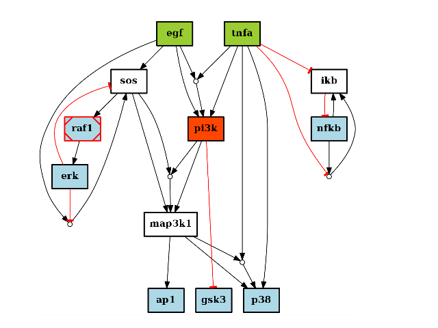
Parameters: kargs – optional arguments accepted by pylab.pcolor From the following graph,
(Source code, png, hires.png, pdf)

The adjacency matrix can be created as follows:
from cno import XCNOGraph, cnodata
c = XCNOGraph(cnodata("PKN-ToyMMB.sif"), cnodata("MD-ToyMMB.csv"))
c.plot_adjacency_matrix()
(Source code, png, hires.png, pdf)

- plot_degree_rank(loc='upper right', alpha=0.8, markersize=10, node_size=25, layout='spring', marker='o', color='b')[source]
Plot degree of all nodes
from cno import XCNOGraph, cnodata
c = XCNOGraph(cnodata("PKN-ToyPB.sif"))
c.plot_degree_rank()
(Source code, png, hires.png, pdf)

- plot_feedback_loops_histogram(**kargs)[source]
Plots histogram of the cycle lengths found in the graph
Returns: list of lists containing all found cycles
- plot_feedback_loops_species(cmap='heat', **kargs)[source]
Returns and plots species part of feedback loops
Parameters: cmap (str) – a color map Returns: dictionary with key (species) and values (number of feedback loop containing the species) pairs. from cno import XCNOGraph, cnodata c = XCNOGraph(cnodata("PKN-ToyPB.sif"), cnodata("MD-ToyPB.csv")) c.plot_feedback_loops_species(cmap='heat', colorbar=True)
(Source code, png, hires.png, pdf)

- plot_in_out_degrees(show=True, ax=None, kind='kde')[source]
from cno import XCNOGraph, cnodata
c = XCNOGraph(cnodata("PKN-ToyPB.sif"), cnodata("MD-ToyPB.csv"))
c.plot_in_out_degrees()
(Source code, png, hires.png, pdf)
1.1.3. MIDAS
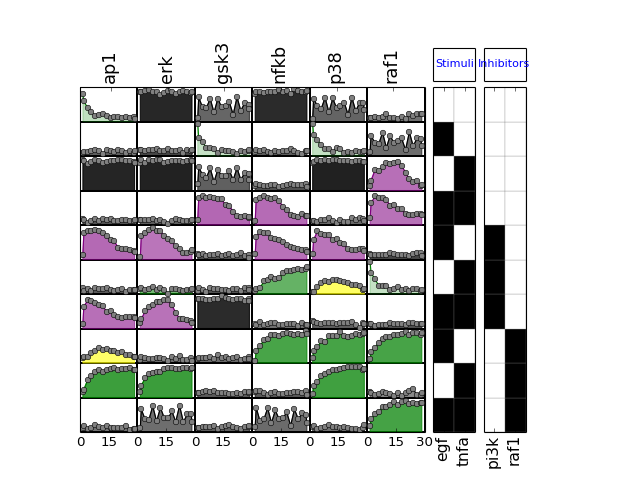
- class XMIDAS(filename=None, cellLine=None, verbose=False, exclude_rows={})[source]
The extended MIDAS data structure.
from cno import XMIDAS, cnodata
m = XMIDAS(cnodata("MD-ToyPB.csv"))
m.df            # access to the data frame
m.experiments   # access to experiments
m.sim           # access to simulation
m.plot()
(Source code, png, hires.png, pdf)

Please see main documentation for extended explanation and documentation of the methods here below.
Warning
if there are replicates, call average_replicates before creating a simulation or calling plot”mode=”mse”)
When reading a MIDAS file with several cell lines, all data is stored but only one cell line can be visualised and manipulated at a time:
# when reading, you must give the cell line name you want to activate
multiple_cell = XMIDAS('somedata', 'cell1')
# valid cell line names are stored in this attribute
multiple_cell.cellLines
# activating another cell line needs to set this attribute:
multiple_cell.cellLine = 'cell2'
Constructor
Parameters: - filename (str) – filename of a MIDAS file or a XMIDAS instance
- cellLine (str) – name of a cell Line (compulsory if several cell lines are present)
- add_gaussian_noise(mu=0, sigma=0.1, inplace=False)[source]
add gaussian noise to the data. Results may be negative or above 1
Parameters: - beta (float) – see equation
- sigma (float) – see equation (default to 0.1)
- inplace (bool) – Default to False
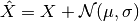
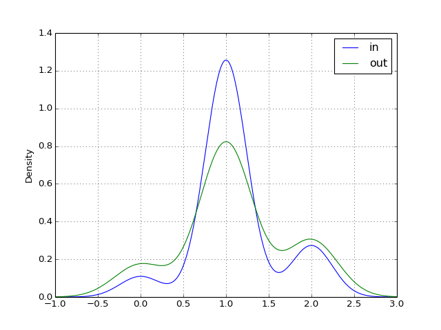
- add_uniform_distributed_noise(inplace=False, dynamic_range=1, mode='bounded')[source]
add random (uniformaly distributed) noise to the dataframe
The noise is uniformly distributed between -0.5 and 0.5 and added to the values contained in the dataframe (for each combinaison of species and time/experiment). New values are
 ,
where dr is the dynamical range. Note that final values may be below
zero or above 1. If you do not want this feature, set the mode to
“bounded” (The default is free). bounded means
,
where dr is the dynamical range. Note that final values may be below
zero or above 1. If you do not want this feature, set the mode to
“bounded” (The default is free). bounded meansParameters: - inplace (bool) – False by default
- dynamic_range (float) – a multiplicative value set to the noise
- mode (str) – bounded (between min and max of the current data) or free
- average_replicates(inplace=False)[source]
Average replicates if any
Parameters: inplace (bool) – default to False If inplace, a new dataframe errors is created and contains the errors (standard deviation)
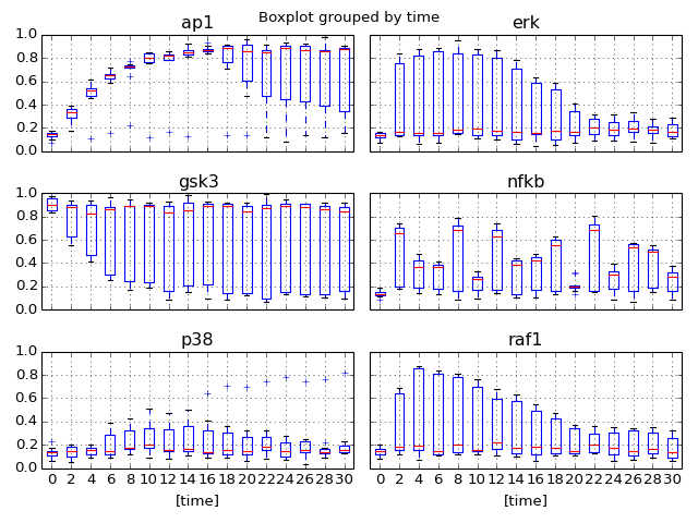
- boxplot(mode='time')[source]
Plot boxplot of the dataframe with the data
Parameters: mode (str) – time or species
- cellLine
Getter/Setter of the active cell line
- cellLines
Return available cell lines
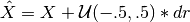
- corr(names=None, cmap='gist_heat_r', show=True)[source]
plot correlation between the measured species
Parameters: - names (list) – restriction to some species if provided.
- cmap (string) – a valid colormap (e.g. jet). Can also use “green” or “heat”.
>>> from cno import XMIDAS, cnodata
>>> m = XMIDAS(cnodata("MD-ToyPB.csv"))
>>> m.corr(cmap="green")
(Source code, png, hires.png, pdf)
- create_empty_simulation()[source]
Populate the simulation dataframe with zeros.
The simulation has the same layout as the experiment.
The dataframe is stored in sim.
- create_random_simulation()[source]
Populate the simulation dataframe with uniformly random values.
The simulation has the same layout as the experiment.
The dataframe is stored in sim.
- discretise(inplace=True, N=2)[source]
Discretise data by rounding up the values
Parameters: - N (int) – number of discrete values (defaults to 2). If set to 2, values will be either 0 or 1. If set to 5, values wil lbe in [0,0.25,0.5,0.75,1]
- inplace –
- experiments
Return dataframe with experiments
- get_diff(sim=None, squared=True, normed=True)[source]
Return dataframe with differences between the data and simulation
The dataframe returned contains the MSE (mean square error) by default.
Parameters: - sim – if not provided, uses the sim attribute.
- normed –
- square (bool) – set to True to get MSE otherwise, returns the absolute values without squaring
if square is True and normed is True:
We then sum over time and if normed is False,
 is set to 1.
- get_max_errors(level='time', normed=False)[source]
Returns max error possible
Should be below one once normalised but could be as low as 0.5
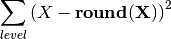
- get_residual_errors(level='time', normed=False)[source]
Return vector with residuals errors
The residual errors are interesting to look at in the context of a boolean analysis. Indeed, residual errors is the minimum error that is unavoidable with a boolean network and comes from the discrete nature of such a model. In a boolean analysis, one would compare 0/1 values to continuous values between 0 and 1. Therefore, however good is the optimisation, the value of the goodness of fit term cannot go under this residual error.
Param: level to sum over Returns: a time series with summed residual errors 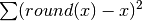 the summation is performed over species
and experiment by default.
the summation is performed over species
and experiment by default.>>> from cno import cnodata, XMIDAS >>> m = XMIDAS(cnodata("MD-ToyMMB_T2.csv")) >>> m.get_residual_errors() time 0 0.000000 10 2.768152 100 0.954000 dtype: float64
if normed is False, returns:
where level can be either over time or experiment. If normed is True, divides the time series by number of experiments and number of times
Note
if normed set to False, same results as in CellNOptR for mode set to time.
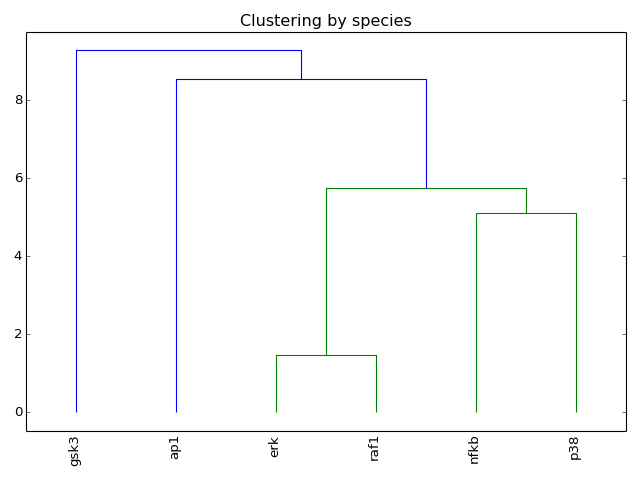
- hcluster(mode='experiment', metric='euclidean', leaf_rotation=90, leaf_font_size=12, **kargs)[source]
Plot the hiearchical cluster (simple approach)
from cno import XMIDAS, cnodata
m = XMIDAS(cnodata("MD-ToyPB.csv"))
m.hcluster("species")
(Source code, png, hires.png, pdf)
- heatmap(cmap='heat', transpose=False)[source]
Hierarchical clustering on species and one of experiment/time level
from cno import XMIDAS, cnodata
m = XMIDAS(cnodata("MD-ToyPB.csv"))
m.heatmap()
(Source code, png, hires.png, pdf)
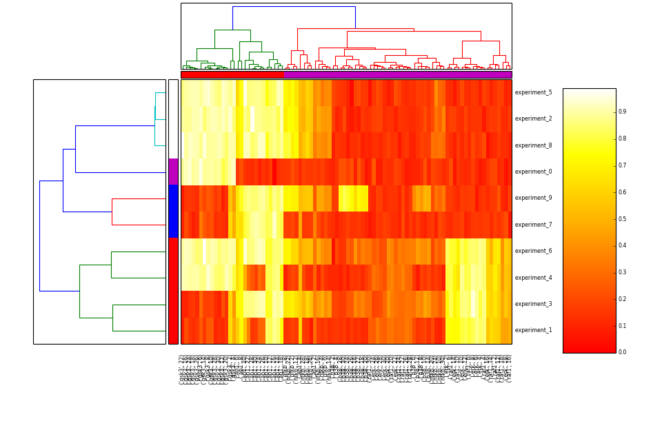
Note
time zero is ignored. Indeed, data at time zero is mostly set to zero, which biases clustering.
- imshow(time, colorbar=True, cmap=None, vmin=None, vmax=None, edgecolors='k')[source]
vmax and vmin are replaced so that we have a symmetric colorbar centered around 0
- inhibitors
return the inhibitors dataframe
- nExps
return number of experiments
- nSignals
return the number of signals
- names_cues
Return list of stimuli and inhibitors together
- names_inhibitors
return list of inhibitors
- names_signals
same as names_species
- names_species
list of species
- names_stimuli
returns list of stimuli
- normalise(mode, inplace=True, changeThreshold=0, **kargs)[source]
Normalise the data
Parameters: - mode – ‘time’ or ‘control’
- inplace (bool) – Defaults to True.
Warning
not fully tested. the mode “time” should work. The control mode has been tested on 2 MIDAS files only. This is a complex normalisation described in XMIDASNormalise
- pca(pca_components=2, fontsize=16)[source]
PCA analysis
from cno import XMIDAS, cnodata
m = XMIDAS(cnodata("MD-ToyPB.csv"))
m.pca()
(Source code, png, hires.png, pdf)

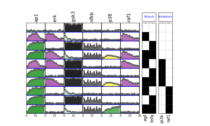
- plot(mode='data', **kargs)[source]
Plot data contained in experiment and df dataframes.
Parameters: - mode (string) – must be either “mse” or “data” (defaults to data)
- fignum – figure number
if mode is ‘mse’, calls also plot_layout, plot_data and plot_sim_data else calls plot_layout and plot_data
from cno import XMIDAS, cnodata
m = XMIDAS(cnodata("MD-ToyPB.csv"))
m.plot(mode="mse")
(Source code, png, hires.png, pdf)

- plot_data(logx=False, color='black', **kargs)[source]
plot experimental curves
>>> from cno import XMIDAS, cnodata
>>> m = XMIDAS(cnodata("MD-ToyPB.csv"));
>>> m.plot_layout()
>>> m.plot_data()
(Source code, png, hires.png, pdf)

Note
called by plot()
See also
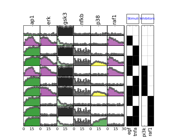
- plot_layout(cmap='heat', rotation=90, colorbar=True, vmax=None, vmin=0.0, mode='data', **kargs)[source]
plot MSE errors and layout
Parameters: - cmap –
- rotation –
- colorbar –
- vmax –
- vmin –
- mode –
- fignum (int) – figure number
>>> from cno import cnodata, XMIDAS
>>> m = XMIDAS(cnodata("MD-ToyPB.csv"));
>>> m.plot_layout()
(Source code, png, hires.png, pdf)

Note
called by plot()
See also
- plot_mse(mode='mse', cmap='heat', vmax=1, vmin=0, hold=False)[source]
Simpler and faster version of plot() function
- plot_sim_data(markersize=3, logx=False, linestyle='--', marker='x', **kargs)[source]
plot experimental curves
>>> from cno import XMIDAS, cnodata
>>> m = XMIDAS(cnodata("MD-ToyPB.csv"))
>>> m.plot_layout()
>>> m.plot_data()
>>> m.plot_sim_data()
(Source code, png, hires.png, pdf)
- radviz(species=None, fontsize=10)[source]
from cno import XMIDAS, cnodata
m = XMIDAS(cnodata("MD-ToyPB.csv"))
m.radviz(["ap1", "gsk3", "p38"])
(Source code, png, hires.png, pdf)

- read()
- remove_experiments(labels)[source]
Remove experiment(s) from the dataframe
Parameters: labels (list) – one experiment or a list of experiments. Valid experiments are in the experiments.index dataframe. Experiments are of the form “experiment_12”. You can refer to an experiment by its number (e.g., here 12).
- remove_inhibitors(labels)[source]
Remove inhibitor(s) from the experiment dataframe
Parameters: labels – a string or list of string representing the inhibitor(s)
- remove_species(labels)[source]
Remove a set of species
Parameters: labels – list of Species (list of strings) or just one species(single string or as a list. m.remove_species("p38") m.remove_species(["p38"])
- remove_stimuli(labels)[source]
Remove a stimuli from the experiment dataframe
Parameters: labels – a string or list of string representing the stimuli
- remove_times(labels)[source]
Remove time values from the data
Parameters: labels (list) – one time point or a list of time points. Valid time points are in the times attribute.
- rename_cellLine(to_replace)[source]
Rename cellLine indices
Parameters: to_replace (dict) – dictionary with mapping of values to be replaced. For example; to rename a valid cell line use:
m.rename_cellLine({"undefined": "PriHu"})
- rename_experiments(to_replace)[source]
Rename experiments in the df and experiments dataframes
Parameters: to_replace (dict) – a dictionary mapping old values (key) to new values (value)
- rename_inhibitors(names_dict)[source]
Rename inhibitors
Parameters: names_dict – a dictionary with names (keys) to be replaced (values) from cno import XMIDAS, cnodata m = XMIDAS(cnodata("MD-ToyPB.csv")) m.rename_species({"raf":"RAF"})
See also
- rename_species(names_dict)[source]
Rename species in the main df dataframe
Parameters: names_dict – a dictionary with names (keys) to be replaced (values) from cno import cnodata, XMIDAS m = XMIDAS(cnodata("MD-ToyPB.csv")) m.rename_species({"erk":"ERK", "akt":"AKT"})
See also
- rename_stimuli(names_dict)[source]
Rename stimuli in the experiment dataframe
Parameters: names_dict – a dictionary with names (keys) to be replaced (values) from cno import XMIDAS, cnodata m = XMIDAS(cnodata("MD-ToyPB.csv")) m.rename_species({"erk":"ERK", "akt":"AKT"})
See also
- rename_time(to_replace)[source]
Rename time indices
Parameters: to_replace (dict) – dictionary with mapping of values to be replaced. For example; to convert time in minutes to time in seconds, use something like:
m.rename_time({0:0,1:1*60,5:5*60})
- reset_experiments()[source]
remove duplicated experiments and rename them from 0 to N
If experiments are duplicated for some reasons (e.g., you removed an entire column with a given inibitor), then experiments may be duplicated. In which case, you may want to (1) remove the duplicated experiments (2) rename the name so that it goes from 0 to the new number of unique experiments and (3) reflect those changes into the df dataframe.
There could be replicares in the resulting df attribute, which should be averaged by the user using average_replicates() method.
- reset_index()[source]
Remove all indices (cellLine, time, experiment)
Done in the 3 dataframes df, sim and errors
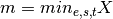
- scale_max(inplace=True)[source]
Divide all data by the maximum over the entire data set

where
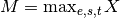 (with
(with  the experiment,
 the species, and
  the time).
- scale_max_across_experiments(inplace=True)[source]
Rescale each species column across all experiments

In the MIDAS plot, this is equivalent to dividing each column by the max over that column. So, on each column, you should get 1 max values set to 1 (if the max is unique). The minimum values may not be set to 0.
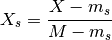
- scale_min_max(inplace=True)[source]
Divide all data by the maximum over entire data set
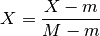
where
 and
and 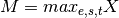 ,
with the experiment, with the species,
with the time.
,
with the experiment, with the species,
with the time.This is an easy (but naive way) to set all data points between 0 and 1.
- scale_min_max_across_experiments(inplace=True)[source]
Rescale each species column across all experiments
where
and ,
with the experiment, with the species,
with the time.
- set_index()[source]
Reset all indices (cellLine, time, experiment)
Done in the 3 dataframes df, sim and errors
- shuffle(mode='experiment', inplace=True)[source]
Shuffle data
This method does not alter the data but shuffles it depending on the user choice.
Parameters: - mode (str) – type of shuffling (see below)
- inplace (bool) – Defaults to True
The mode parameter can be
- timeseries shuffles experiments and species; timeseries
are unchanged.
- all: through times, experiments and species. No structure kept
sum of the data is constant.
signal (or species or column): within a column, timeseries are shuffled. So, sum over signals is constant.
experiment (or index): with a row (experiment), timeseries are shuffled. Sum of data over a row is constant.
Original data:
(Source code, png, hires.png, pdf)
Shuffling all timeseries (shuffling rows and columsn in the plot):
from cno import XMIDAS, cnodata
m = XMIDAS(cnodata("MD-ToyPB.csv"))
m.shuffle(mode="timeseries")
m.plot()
(Source code, png, hires.png, pdf)
Warning
shuffling is made inplace.
- signals
Getter for the columns of the dataframe that represents the species/signals
- sort_experiments_by_inhibitors()[source]
Sort the experiments by inhibitors
Affects the experiment dataframe for th rendering but do not change the dataframe that contains the data.
- sort_experiments_by_stimuli()[source]
Sort experiments by stimuli
Affects the experiment dataframe for th rendering but do not change the dataframe that contains the data.
- species
Getter for the columns of the dataframe that represents the species/signals
- stimuli
return the stimuli dataframe
- times
Getter to the different times
- to_measurements()[source]
Returns a Measurements instance
Each datum in the dataframe df is converted into an instance of Measurements.
Returns: list of experiments. mb = MIDASbuilder(m.to_measurements) mb.xmidas

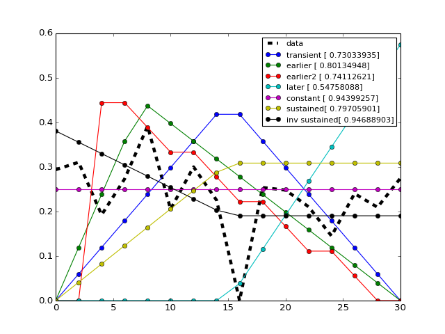
- class Trend[source]
Utility that figures out the trend of a time series
from cno import cnodata
from cno.io import midas

# get a time series
xm = midas.XMIDAS(cnodata("MD-ToyPB.csv"))
ts = xm.df['ap1']['Cell']['experiment_0']

# set a trend instance
trend = midas.Trend()
trend.set(ts)
trend.plot()

trend.get_bestfit_color()
(Source code, png, hires.png, pdf)
- alpha
return strength of the signal
- normed_times
return normed time array
- normed_values
return normed value array
- times
return time array
- values
return the value array
- class MIDASReader(filename, verbose='ERROR', exclude_rows={})[source]
A MIDAS reader that converts the experiments and data into dataframes
Used by XMIDAS to read and convert the data.
CellLine must be encoded in the header as follows:
TR:name:CellLine
If name is not provided, it is replaced internally with “undefined”.
Those columns are ignored in MIDASReader:
[‘NOINHIB’, ‘NOCYTO’, ‘NOLIG’, ‘NO-CYTO’, ‘NO-INHIB’, ‘NO-LIG’]User should not need to use this class. Use XMIDAS instead.
This is an experimental module to design an XML format for MIDAS data sets.
- class XMLMIDAS(filename)[source]
Class to read MIDAS in XML format.
- xmidas
Get XMIDAS instance from the XML
- class Measurement(protein_name, time, stimuli, inhibitors, value, cellLine=u'undefined', units=u'second')[source]
Data structure to store a measurement.
Givem a list of stimuli and inhibitor, stores a measure at a given time.
>>> from cno.io.midas_extra import Measurement
>>> m = Measurement("AKT", 0, {"EGFR":1}, {"AKT":0}, 0.1)
Parameters: - protein (str) –
- time (float) –
- stimuli (dict) – a dictionary
- inhibitors (dict) – a dictionary
- measurement (float) – the value
- cellLine (str) – Defaults to “undefined”
- units (str) – Defaults to “second” (not yet used)
- cellLine
- data
- inhibitors
- protein_name
- stimuli
- time
- units
units (second, hour, minute, day
- class Measurements(measurements=None)[source]
Data structure to store list of measurements
>>> es = Measurements()
>>> e1 = Measurement("AKT", 0, {"EGFR":1}, {"AKT":0}, 0.1)
>>> e2 = Measurement("AKT", 5, {"EGFR":1}, {"AKT":0}, 0.5)
>>> es.add_measurements([e1,e2])
- append()
L.append(object) – append object to end
- count(value) → integer -- return number of occurrences of value
- extend()
L.extend(iterable) – extend list by appending elements from the iterable
- index(value[, start[, stop]]) → integer -- return first index of value.
Raises ValueError if the value is not present.
- inhibitors
- insert()
L.insert(index, object) – insert object before index
- pop([index]) → item -- remove and return item at index (default last).
Raises IndexError if list is empty or index is out of range.
- remove()
L.remove(value) – remove first occurrence of value. Raises ValueError if the value is not present.
- reverse()
L.reverse() – reverse IN PLACE
- sort()
L.sort(cmp=None, key=None, reverse=False) – stable sort IN PLACE; cmp(x, y) -> -1, 0, 1
- species
- stimuli
- class MIDASBuilder[source]
STarts a MIDAS file from scratch and export 2 CSV MIDAS file.
Warning
to be used with care. Right now it seems to work but still in development.
>>> m = MIDASBuilder()
>>> e1 = Measurement("AKT", 0, {"EGFR":1}, {"AKT":0}, 0.1)
>>> e2 = Measurement("AKT", 5, {"EGFR":1}, {"AKT":0}, 0.5)
>>> e3 = Measurement("AKT", 10, {"EGFR":1}, {"AKT":0}, 0.9)
>>> e4 = Measurement("AKT", 0, {"EGFR":0}, {"AKT":0}, 0.1)
>>> e5 = Measurement("AKT", 5, {"EGFR":0}, {"AKT":0}, 0.1)
>>> e6 = Measurement("AKT", 10, {"EGFR":0}, {"AKT":0}, 0.1)
>>> for e in [e1, e2, e3, e4, e5, e6]:
...     m.add_measurement(e)
>>> m.to_midas("test.csv")
This class allows one to add measurements to obtain a dataframe compatible with XMIDAS class, which can then be saved using XMIDAS.to_midas.
If an inhibitor or stimuli is not provided, we assume ti is absent (set to zero).
- inhibitors
- stimuli
- test_example(Nspecies=20, N=10, times=[0, 10, 20, 30])[source]
N number of stimuli and inhibitors Ntime = There are duplicates so Nrows = N*2 * Ntimes * 2
- xmidas
1.1.4. Reactions
This module contains a base class to manipulate reactions
- class Reaction[source]
Logical Reaction
A Reaction can encode logical ANDs and ORs as well as NOT:
>>> from cno import Reaction
>>> r = Reaction("A+B=C") # a OR reaction
>>> r = Reaction("A^B=C") # an AND reaction
>>> r = Reaction("A&B=C") # an AND reaction
>>> r = Reaction("C=D")   # an activation
>>> r = Reaction("!D=E")  # a NOT reaction
The syntax is as follows:
- The ! sign indicates a logical NOT.
- The + sign indicates a logical OR.
- The = sign indicates a relation (edge).
- The ^ or & signs indicate a logical AND. Note that & signs will be replaced by ^.
Internally, reactions are checked for validity (e.g., !=C is invalid).
You can reset the name:
>>> r.name = "A+B+C=D"
or create an instance from another instance:
>>> newr = Reaction(r)
Sorting can be done inplace (default) or not.
>>> r = Reaction("F+D^!B+!A=Z")
>>> r.sort(inplace=False)
'!A+!B^D+F=Z'
Simple operator (e.g., equality) are available. Note that equality will sort the species internally so A+B=C would be equal to B+A=C and there is no need to call sort():
>>> r = Reaction("F+D^!B+!A=Z")
>>> r == '!A+!B^D+F=Z'
True
If a reaction A+A=B is provided, it can be simplified by calling simplify(). ANDs operator are not simplified. More sophisticated simplifications using Truth Table could be used but will not be implemented in this class for now.
- lhs
Getter for the left hand side of the = character
- lhs_species
Getter for the list of species on the left hand side of the = character
- name
Getter/Setter for the reaction name
- rhs
Getter for the right hand side of the = character
- sign
return sign of the reaction
- simplify(inplace=True)[source]
Simplifies reaction if possible.
>>> r = Reaction("A+A=B")
>>> r.simplify()
>>> r
"A=B"
Other cases (with ANDs) are not simplified. Even though A+A^B=C truth table could be simplified to A=C but we will not simplified it for now.
- sort(inplace=True)[source]
Rearrange species in alphabetical order
Parameters: inplace (bool) – defaults to True >>> r = Reaction("F+D^!B+!A=Z") >>> r.sort() >>> r '!A+!B^D+F=Z'
- species
>>> r = Reaction("!a+c^d^e^f+!h=b")
>>> r.species
['a', 'c', 'd', 'e', 'f', 'h', 'b']
- class Reactions(reactions=, []strict_rules=True, verbose=False)[source]
Data structure to handle list of Reaction instances
For the syntax of a reaction, see Reaction. You can use the =, !, + and ^ characters.
Reactions can be added using either string or instances of Reaction:
>>> from cno import Reaction, Reactions
>>> r = Reactions()
>>> r.add_reaction("A+B=C") # a OR reaction
>>> r.add_reaction("A^B=C") # an AND reaction
>>> r.add_reaction("A&B=C") # an AND reaction
>>> r.add_reaction("C=D")   # an activation
>>> r.add_reaction("!D=E")  # a NOT reaction
>>> r.add_reaction(Reaction("F=G"))  # a NOT reaction
Now, we can get the species:
>>> r.species
['A', 'B', 'C', 'D', 'E']
Remove one:
>>> r.remove_species("A")
>>> r.reactions
["B=C", "C=D", "!D=E"]
Note
there is no simplifications made on reactions. For instance, if you add A=B and then A+B=C, A=B is redundant but will be kept.
See also
- add_reaction(reaction)[source]
Adds a reaction in the list of reactions
See documentation of the Reaction class for details. Here are some valid reactions:
a=b
a+c=d
a^b=e  # same as above
!a=e
Example:
>>> from cno import Reactions
>>> c = Reactions()
>>> c.add_reaction("a=b")
>>> assert len(c.reactions) == 1
- add_reactions(reactions)[source]
Add a list of reactions
Parameters: reactions (list) – list of reactions or strings
- reactions
return list of reaction names
- remove_reaction(reaction_name)[source]
Remove a reaction from the reacID list
>>> c = Reactions()
>>> c.add_reaction("a=b")
>>> assert len(c.reactions) == 1
>>> c.remove_reaction("a=b")
>>> assert len(c.reactions) == 0
- remove_species(species_to_remove)[source]
Removes species from the list of reactions
Parameters: species_to_remove (str,list) – Note
If a reaction is “a+b=c” and you remove specy “a”, then the reaction is not enterely removed but replace by “b=c”
- rename_species(mapping={})[source]
Rename species in all reactions
Parameters: mapping (dict) – The mapping between old and new names
- search(species, strict=False)[source]
Prints and returns reactions that contain the species name
Parameters: - species (str) – name to look for
- strict (bool) – decompose reactions to search for the species
Returns: a Reactions instance with reactions containing the species to search for
- species
return list of unique species
1.1.5. SIF format
- class SIF(filename=None, frmt='cno')[source]
Manipulate network stored in SIF format.
The SIF format is used in Cytoscape and CellNOpt (www.cellnopt.org). However, the format used in CellNOpt(R) restrict edges to be only 1 or -1. Besides, special nodes called AND nodes can be added using the “and” string followed by a unique identifier(integer) e.g., and22; see below for details.
See also
sif section in the online documentation.
The SIF format is a tab-separated format. It encodes relations between nodes in a network. Each row contains a relation where the first column represents the input node, the second value is the type of relation. The following columns represents the output node(s). Here is a simple example:
A 1 B
B 1 C
A -1 B
but it can be factorised:
A 1 B C
B 1 C
In SIF, only OR reactions can be encoded. The following:
A 1 C
B 1 C
means A OR B gives C. AND reactions cannot be encoded therefore we have to code AND gates in a special way using a dedicated syntax. In order to encode the AND reaction the SIF reaction should be encoded as follows:
A 1 and1
B 1 and1
and1 1 C
An AND gate is made of the “and” string and a unique id concatenated as its end.
A SIF file can be read as follows:
s = SIF(filename)
Each line is transformed into reactions (A=B, !A=B). You can then add or remove reactions. If you save the file in a new SIF file, be aware than lines such as:
A 1 B C
are expanded as:
A 1 B
A 1 C
Aliases to the columns are stored in read-only attributes called nodes1, edges, nodes2. You can only add or remove reactions. Reactions are stored in reactions.
Constructor
Parameters: - filename (str) – optional input SIF file.
- frmt (str) – “cno” or “generic” are accepted (default is cno). The cno format accepted only relation as “1” for activation, and “-1” for inhibitions. The “generic” format allows to have any relations. The “cno” format also interprets nodes that starts with “and” as logical AND gates. Such nodes are transformed into more cmpact notations. That is reactions.
A 1 and1
B -1 and1
and1 1 C
is transformed internally as 1 reaction: A^!B=C
- add_reaction(reaction)[source]
Adds a reaction into the network.
Valid reactions are:
A=B
A+B=C
A^B=C
A&B=C
Where the LHS can use as many species as desired. The following reaction is valid:
A+B+C+D+E=F
Note however that OR gates (+ sign) are splitted so A+B=C is added as 2 different reactions:
A=C
B=C
- add_reactions(reactions)
Add a list of reactions
Parameters: reactions (list) – list of reactions or strings
- and_nodes
Returns list of AND nodes
- and_symbol = '^'
- edges
returns list of edges found in the reactions
- nodes1
returns list of nodes in the left-hand sides of the reactions
- nodes2
returns list of nodes in the right-hand sides of the reactions
- plot()[source]
Plot the network
Note
this method uses CNOGraph so AND gates appear as small circles.
- reactions
return list of reaction names
- read_sbmlqual(filename)[source]
import SBMLQual XML file into a SIF instance
Parameters: - filename (str) – the filename of the SBMLQual
- clear (bool) – remove all existing nodes and edges
Warning
experimental
- remove_reaction(reaction_name)
Remove a reaction from the reacID list
>>> c = Reactions()
>>> c.add_reaction("a=b")
>>> assert len(c.reactions) == 1
>>> c.remove_reaction("a=b")
>>> assert len(c.reactions) == 0
- remove_species(species_to_remove)
Removes species from the list of reactions
Parameters: species_to_remove (str,list) – Note
If a reaction is “a+b=c” and you remove specy “a”, then the reaction is not enterely removed but replace by “b=c”
- rename_species(mapping={})
Rename species in all reactions
Parameters: mapping (dict) – The mapping between old and new names
- save(filename)[source]
Save the reactions (sorting with respect to order parameter)
Parameters: filename (str) – where to save the nodes1 edges node2
- search(species, strict=False)
Prints and returns reactions that contain the species name
Parameters: - species (str) – name to look for
- strict (bool) – decompose reactions to search for the species
Returns: a Reactions instance with reactions containing the species to search for
- species
return list of unique species
- to_list()
Return list of reaction names
- to_reactions()[source]
Returns a Reactions instance generated from the SIF file.
AND gates are interpreted. For instance the followinf SIF:
A 1 and1
B 1 and1
and1 1 C
give:
A^B=C
- to_sbmlqual(filename=None)[source]
Exports SIF to SBMLqual format.
Parameters: filename – save to the filename if provided Returns: the SBML text This is a level3, version1 exporter.
>>> s = SIF()
>>> s.add_reaction("A=B")
>>> res = s.to_sbmlqual("test.xml")
Warning
logical AND are not encoded yet. works only if no AND gates
Warning
experimental
- valid_symbols = ['+', '!', '&', '^']
1.1.6. EDA
- class EDA(filename, threshold=0, verbose=False)[source]
Reads networks in EDA format
EDA format is similar to SIF but provides a weight on each edge.
It looks like:
A (1) B = .5
B (1) C =  1
A (1) C = .1
Note
the parentheses and spaces.
Note
no header expected.
Parameters: - filename (str) –
- threshold (float) – should be between 0 and 1 but not compulsary
- verbose (bool) –
- export2sif(threshold=None)[source]
Exports EDA data into SIF file
Parameters: threshold (float) – since EDA format provides a weight on each edge, it can be used as a threshold to consider the relation or not. By default, the threshold is set to 0, which means all edges should be exported in the output SIF format (assuming weights are positive). You ca n either set the threshold attribute to a different value or provide this threshold parameter to override the default threshold. >>> from cno.io.eda import EDA >>> from cno import testing >>> e = EDA(testing.get("test_simple.eda")) >>> s1 = e.export2sif() # default threshold 0 >>> len(s1) 3 >>> s1 = e.export2sif(0.6) # one edge with weight=0.5 is ignored >>> len(s1) 2
1.1.7. CNA
| Topic: | Module dedicated to the CNA reactions data structure |
|---|---|
| Status: | for production but not all features implemented. |
- class CNA(filename=None, type=2, verbose=False)[source]
Reads a reaction file (CNA format)
This class has the Interaction class as a Base class. It is used to read reactions files from the CNA format, which is a CSV-like format where each line looks like:
mek=erk 1 mek = 1 erk | # 0 1 0 436 825 1 1 0.01
The pipe decompose the strings into a LHS and RHS.
The LHS is made of a unique identifier without blanks (mek=erk). The remaining part is the reaction equation. The equal sign “=” denotes the reaction arrow. Identifiers, coefficients and equal sign must be separated by at least one blank. The ! sign to indicate not. The + sign indicates an OR relation.
Warning
The + sign indicates an OR as it should be. However, keep in mind that in CellNOptR code, the + sign indicates an AND gate. In this package we always use + for an OR and ^ or & for an AND gate.
Warning
in the CNA case, some reactions have no LHS or RHS. Such reactions are valid in CNA but may cause issue if converted to SIF
Note
there don’t seem to be any AND in CNA reactions.
The RHS is made of
a default value: # or a value.
- a set of 3 flags representing the time scale
- flag 1: whether this interaction is to be excluded in logical computations
- flag 2: whether the logical interaction is treated with incomplete truth table
- flag 3: whether the interaction is monotone
reacBoxes (columns 5,6,7,8)
monotony (col 9)
In this class, only the LHS are used for now, however, the RHS values are stored in different attributes.
>>> from cno.io import Reactions
>>> from cno import getdata
>>> a = Reactions(getdata('test_reactions'))
>>> reacs = a.reactions
See also
CNA class inherits from cno.io.reaction.Reaction
Constructor
Parameters: - filename (str) – an optional filename containing reactions in CNA format. If not provided, the CNA object is empty but you can add reactions using add_reaction(). However, attributes such as reacBoxes will not be populated.
- type (integer) – only type 2 for now.
- verbose (bool) – False by default
Todo
type1 will be implemented on request.
- excludeInLogical = None
populated when reading CNA reactions file
- incTruthTable = None
populated when reading CNA reactions file
- monotony = None
populated when reading CNA reactions file
- reacBoxes = None
populated when reading CNA reactions file
- reacText = None
populated when reading CNA reactions file
- timeScale = None
populated when reading CNA reactions file
- to_sif(filename=None)[source]
Export the reactions to SIF format
from cno.io import CNA
r = CNA()
r.add_reaction("a=b")
r.add_reaction("a+c=e")
r.to_sif("test.sif")
Again, be aware that “+” sign in Reaction means “OR”. Looking into the save file, we have the a+c=e reactions (a=e OR c=e) expanded into 2 reactions (a 1 e) and (c 1 e) as expected:
a   1   b
a   1   e
c   1   e
1.1.8. Converters
| Topic: | adjacency matrix |
|---|
- class ADJ2SIF(filenamePKN=None, filenameNames=None, delimiter=', ')[source]
Reads an adjacency matrix (and names) from CSV files
Warning
API likely to change to use pandas to simplify the API.
The instance can then be exported to SIF or used as input for the cno.io.cnograph.CNOGraph structure.
>>> from cno.io import ADJ2SIF
>>> from cno import getdata
>>> f1 = getdata("test_adjacency_matrix.csv")
>>> f2 = getdata("test_adjacency_names.csv")
>>> s = ADJ2SIF(f1, f2)
>>> sif = s.to_sif()
>>> c = CNOGraph(s.G)

Where the adjacency matrix looks like::

    0,1,0
    1,0,0
    0,0,1

and names is a 1-column file::

    A
    B
    C

The exported SIF file would look like::

    A 1 B
    A 1 C
Warning
The adjacency matrix contains only ones (no -1) so future version may need to add that information using incidence matrix for instance
Constructor
Parameters: - filenamePKN (str) – adjacency matrix made of 0’s and 1’s.
- filenameNames (str) – names of the columns/rows of the adjacency matrix
- delimiter (str) – commas by default
0,1,0
1,0,0
0,0,1
names:
A
B
C
The 2 files above correspond to this SIF file:
A 1 B
A 1 C
- G
The graph created from the input data
- load_adjacency(filename=None)[source]
Reads an adjacency matrix filename
if no filename is provided, tries to load from the attribute filename.
- names
Names of the nodes read from the the provided filename. Could be empty
| Topic: | convert SIF format to ASP sign consistency |
|---|
- class SIF2ASP(filename=None)[source]
Class to convert a SIF file into a ASP sign consistency format
>>> from cno import SIF2ASP
>>> from cno import cnodata
>>> filename = cnodata("PKN-ToyMMB.sif")
>>> s = SIF2ASP(filename)
>>> s.to_net("PKN-ToyMMB.net")
This module provides tools to convert a SIF file into a format appropriate to check sign consistency with ASP tools:
A 1 B
A -1 C
converted to
A -> B +
A -> C -
See also
This class inherits from cno.io.sif.SIF.
Constructor
Parameters: filename (str) – the SIF filename - signs
get the signs of the reactions
- class SOP2SIF(filename)[source]
Converts a file from SOP to SIF format
SOP stands for sum of products, it is a list of relations of the form:
!A+B=C
For now, this function has been tested and used on the copy/paste of a PDF document into a file. Be careful because the interpretation of the characters may differ from one distribution to the other. The original data contains
- a special character for NOT, which is interpreted as x2xac (a L turned by 90 degrees clockwise)
- an inversed ^ character for OR, which is interpreted as ” _ “
- a ^ character for AND, which is correctly interpreted.
- a -> character for “gives”, which is transformed into ! character.
On other systems, it may be interpreted differently, so we provide a mapping attribute mapping to perform the translation, which can be changed to your needs.
The data looks like:
1 !A + B = C 1 [references]
2 !A + B = E 2 [references]
3 !A + B = D 1 [references]
...
N !A + B = D 2 [references]
The SOP2SIF class gets rid of the last column, the [references] and the column before it (made of 1 and 2). Then, we convert the reaction strings into the same format as in CellNOpt that is:
- A = C means A GIVES C
- A + B = C means A gives C OR B gives C
- !A means NOT A
>>> s2s = SOP2SIF("data.sop")
>>> s = s2s.sop2sif()
>>> s2s.writeSIF("data.sif")
- add_reaction(reaction)
Adds a reaction in the list of reactions
See documentation of the Reaction class for details. Here are some valid reactions:
a=b
a+c=d
a^b=e  # same as above
!a=e
Example:
>>> from cno import Reactions
>>> c = Reactions()
>>> c.add_reaction("a=b")
>>> assert len(c.reactions) == 1
- add_reactions(reactions)
Add a list of reactions
Parameters: reactions (list) – list of reactions or strings
- and_symbol = '^'
- export2sif(filename, include_and_gates=True)[source]
Save the reactions in a file using SIF format
The data read from the SOP file is transformed into a SIF class before hand.
Parameters: include_and_gates (bool) – if set to False, all reactions with AND gates removed
- mapping = None
The dictionary to map SOP special characters e.g if you code NOT with ! character, just fill this dictionary accordingly
- reactions
return list of reaction names
- remove_reaction(reaction_name)
Remove a reaction from the reacID list
>>> c = Reactions()
>>> c.add_reaction("a=b")
>>> assert len(c.reactions) == 1
>>> c.remove_reaction("a=b")
>>> assert len(c.reactions) == 0
- remove_species(species_to_remove)
Removes species from the list of reactions
Parameters: species_to_remove (str,list) – Note
If a reaction is “a+b=c” and you remove specy “a”, then the reaction is not enterely removed but replace by “b=c”
- rename_species(mapping={})
Rename species in all reactions
Parameters: mapping (dict) – The mapping between old and new names
- search(species, strict=False)
Prints and returns reactions that contain the species name
Parameters: - species (str) – name to look for
- strict (bool) – decompose reactions to search for the species
Returns: a Reactions instance with reactions containing the species to search for
- sop2sif(include_and_gates=True)[source]
Converts the SOP data into a SIF class
Parameters: include_and_gates (bool) – if set to False, all reactions with AND gates are removed. Returns: an instance of cno.io.sif.SIF
- species
return list of unique species
- to_list()
Return list of reaction names
- valid_symbols = ['+', '!', '&', '^']
2. MISC
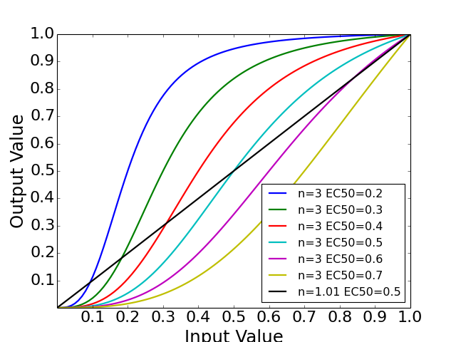
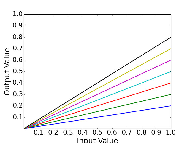
- normhill_tf(x, k, n, g=1)[source]
Return the normalised Hill transfer function
Parameters: - x (array) – Level of input data (from 0 to 1)
- n (float) – the Hill coefficient sharpness of the sigmoidal transition between high and low output node values
- k (float) – is the sensitivity parameter specyfying the EC50 value
- g (float) – a factor
![[source]](_modules/cno/io/cnograph.html#CNOGraph.png)
![[source]](_modules/cno/io/cnograph.html#CNOGraph.svg)
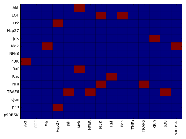
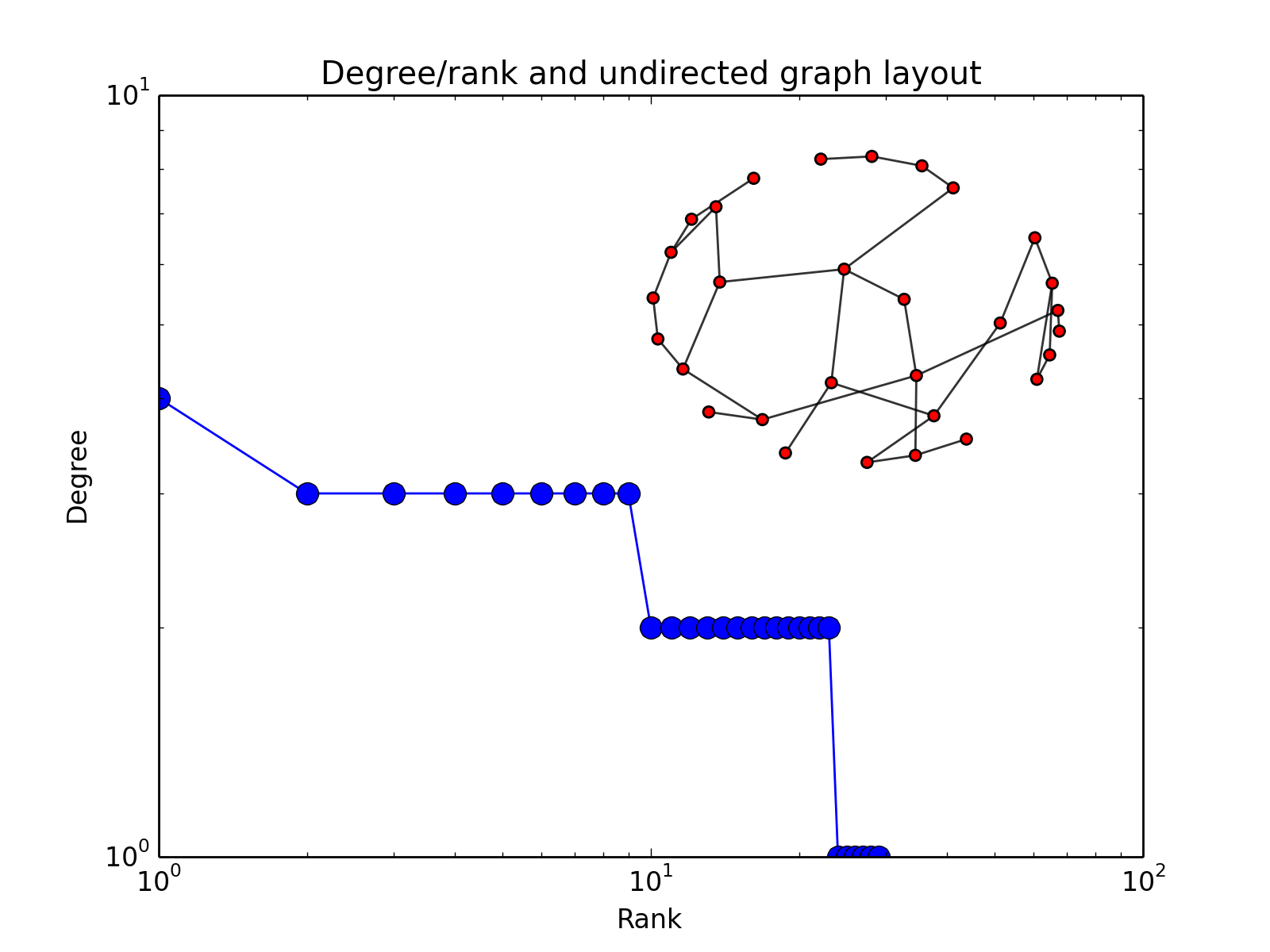
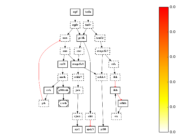
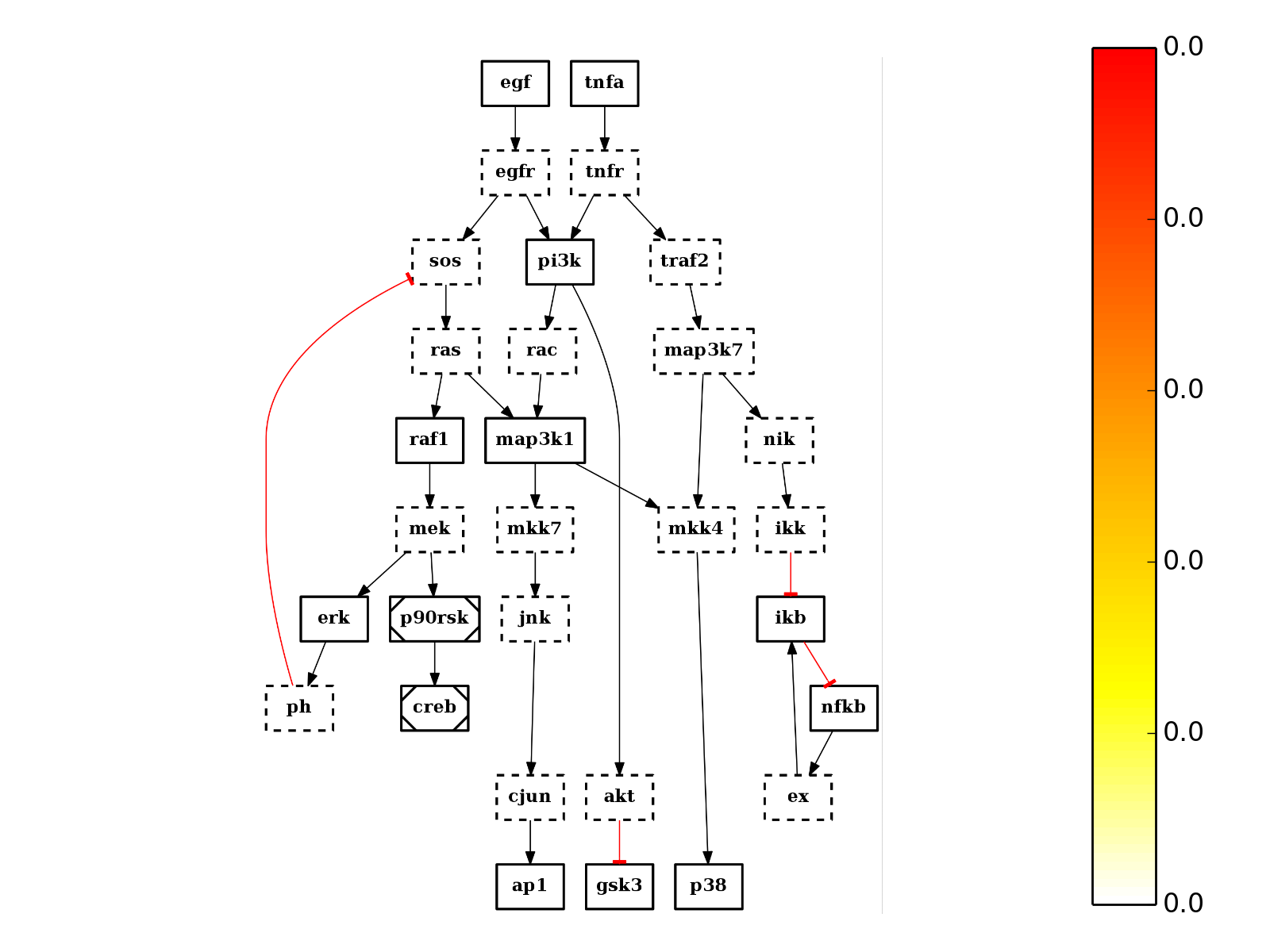
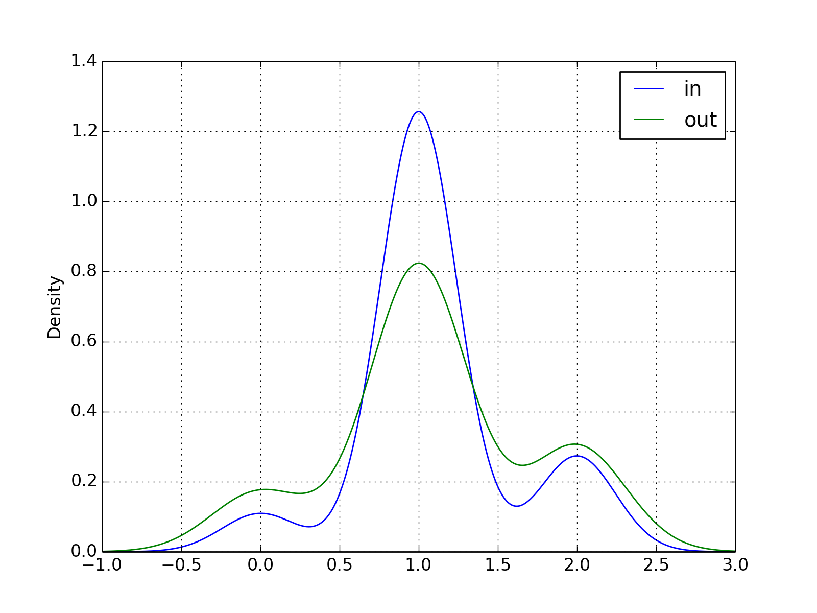
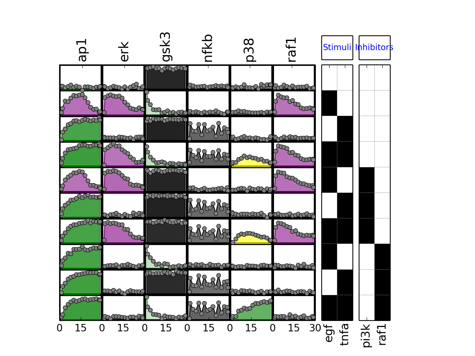
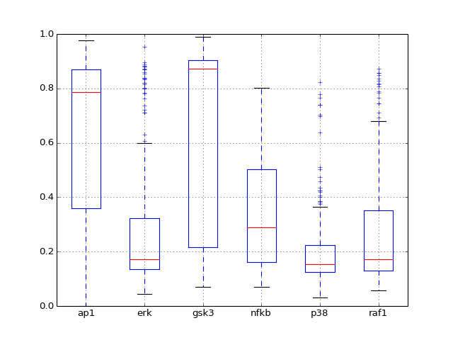
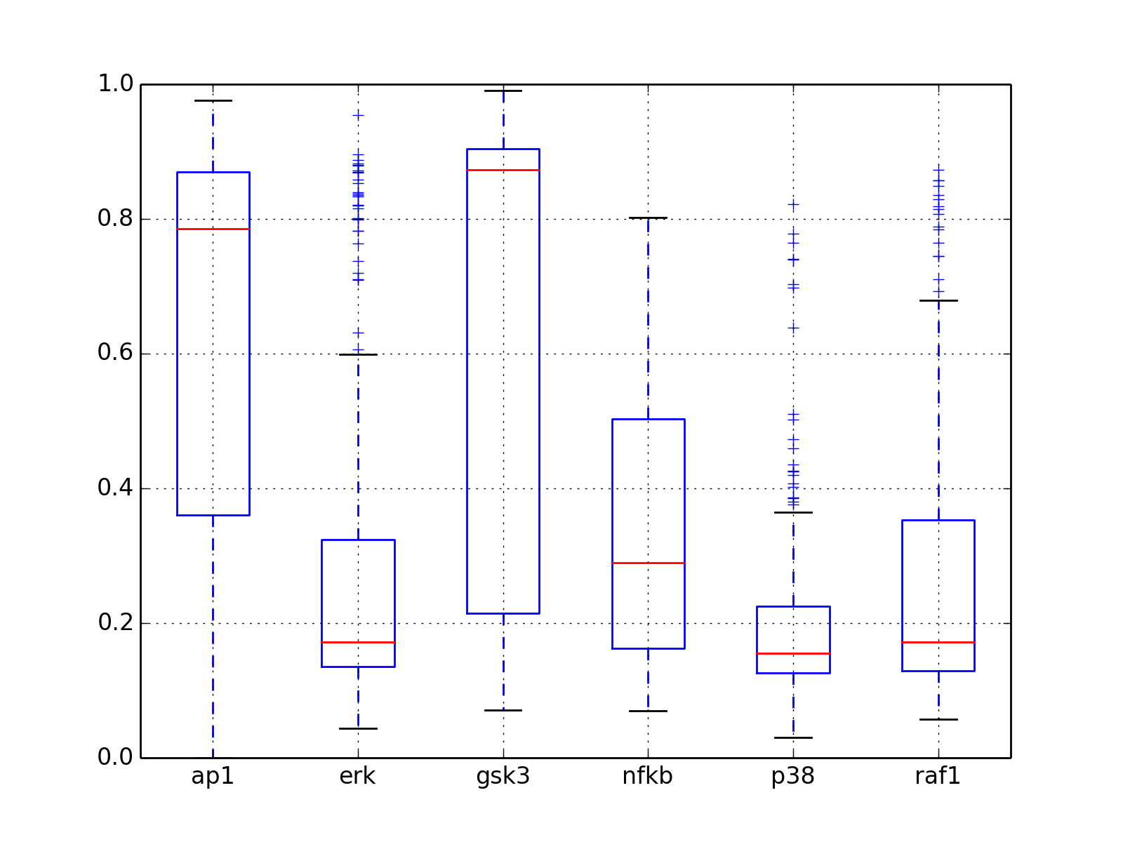
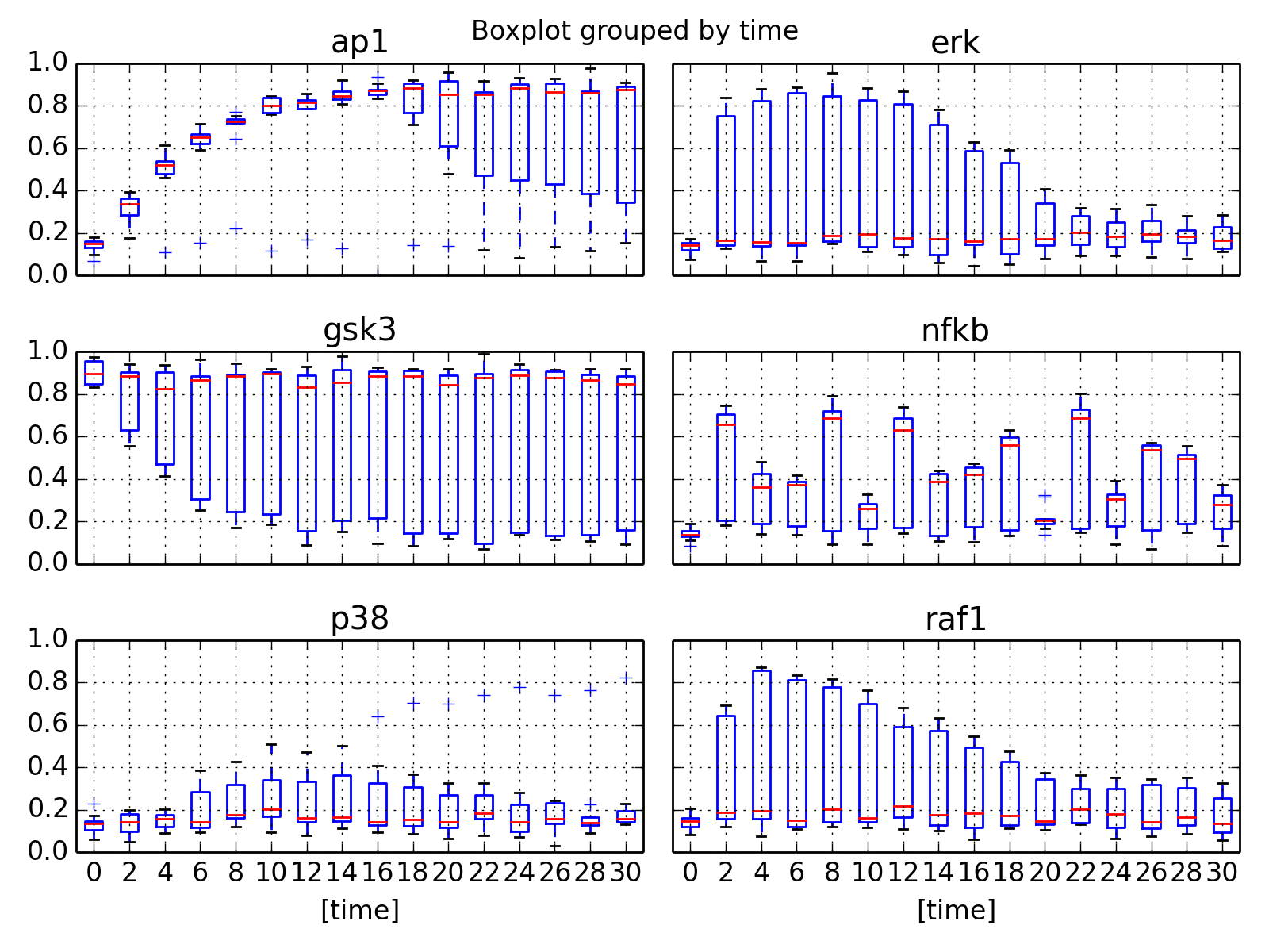
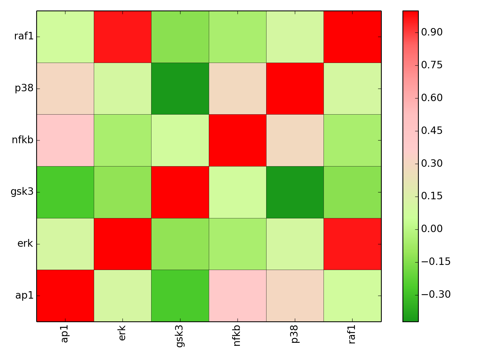
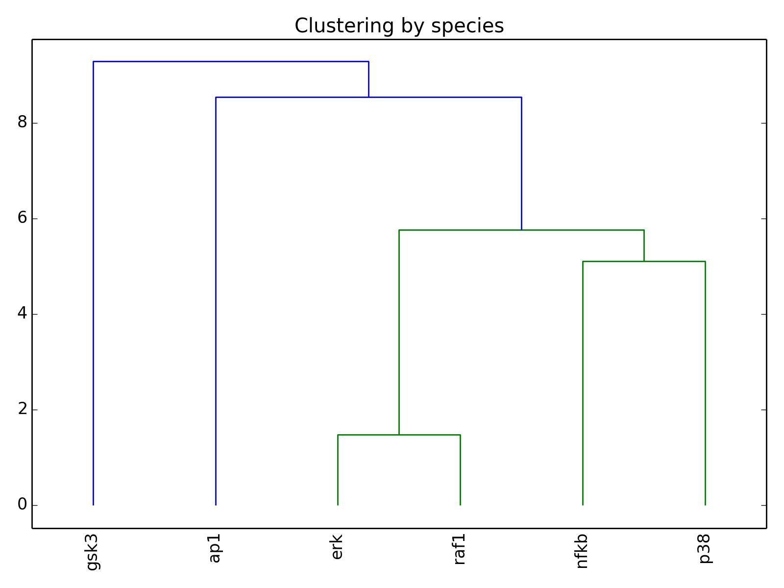
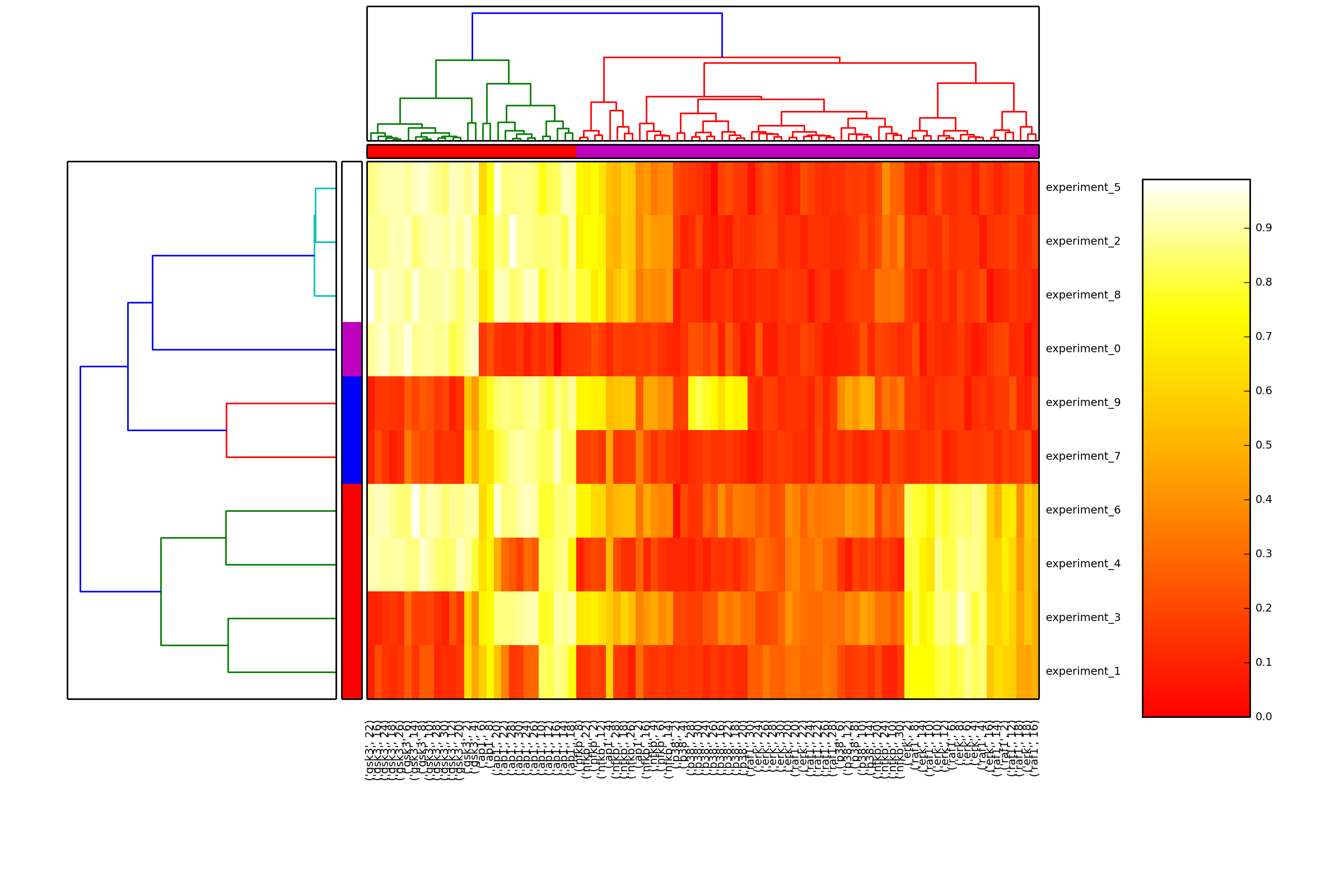
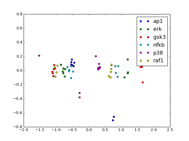
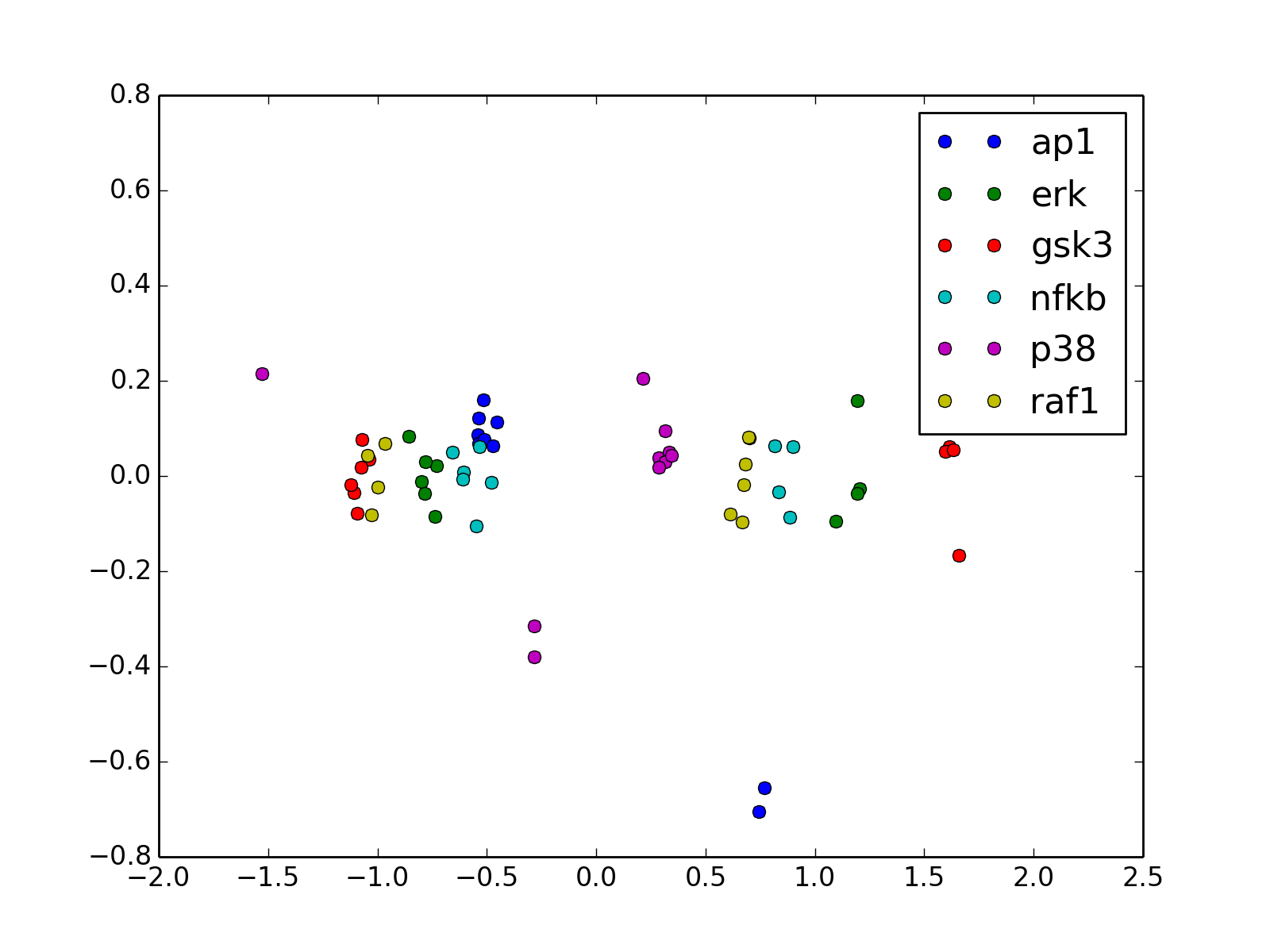
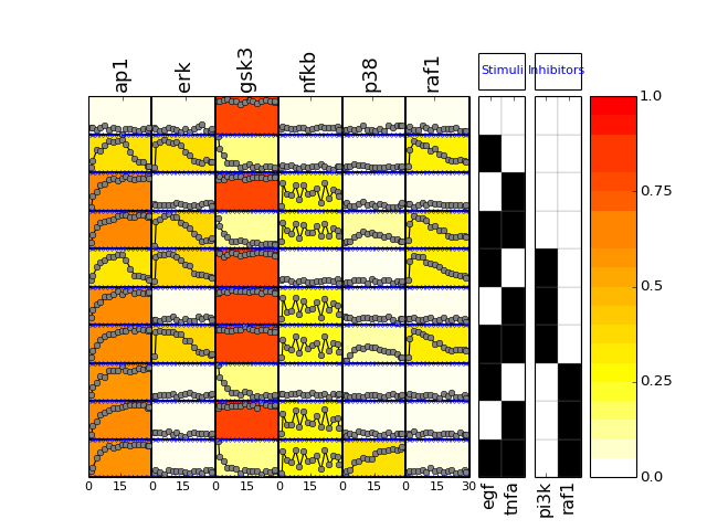
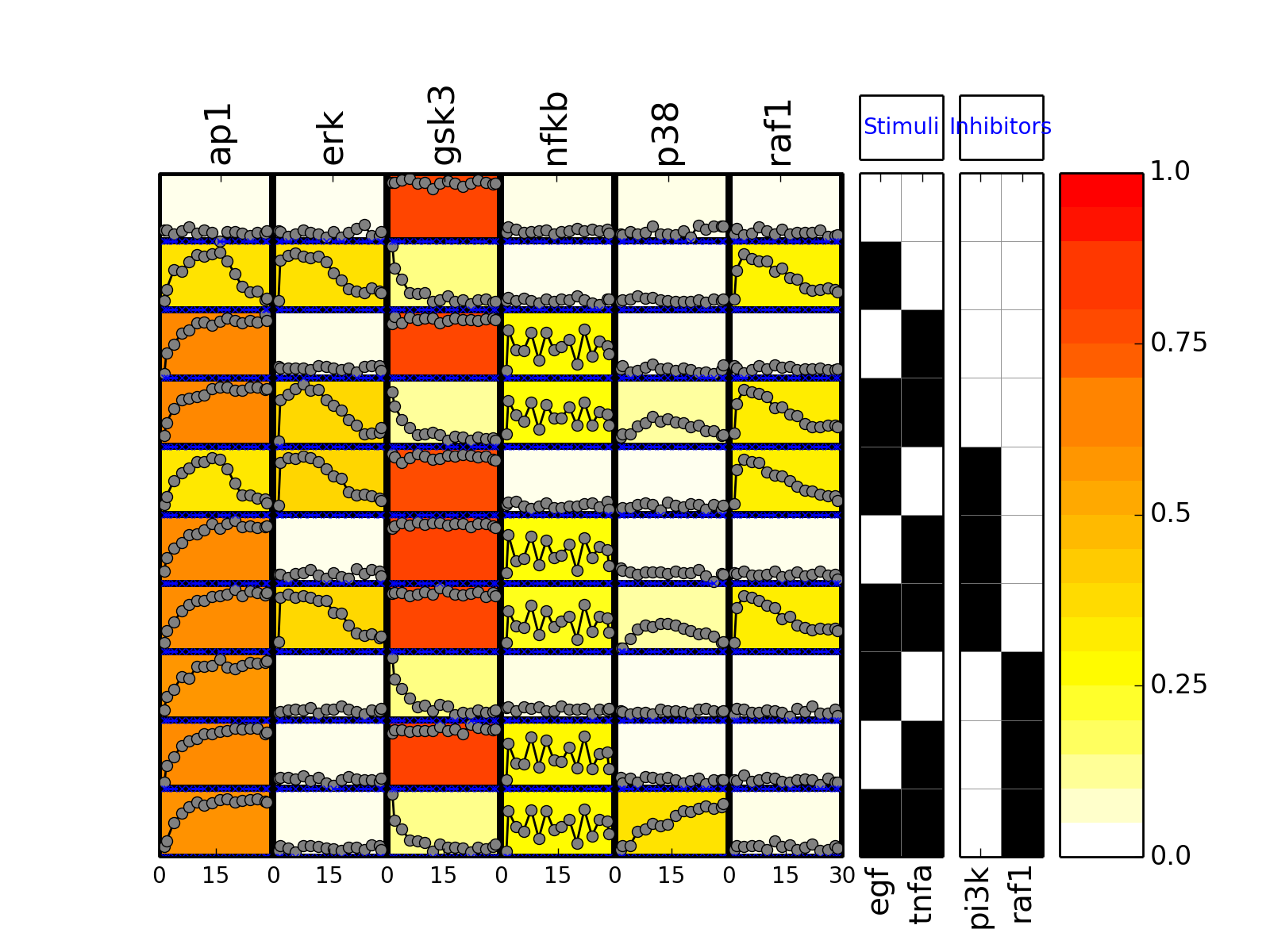
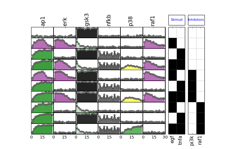
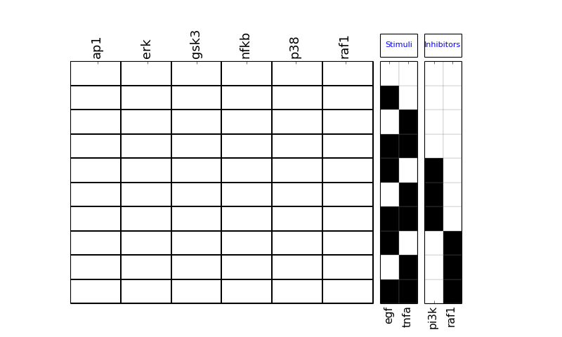
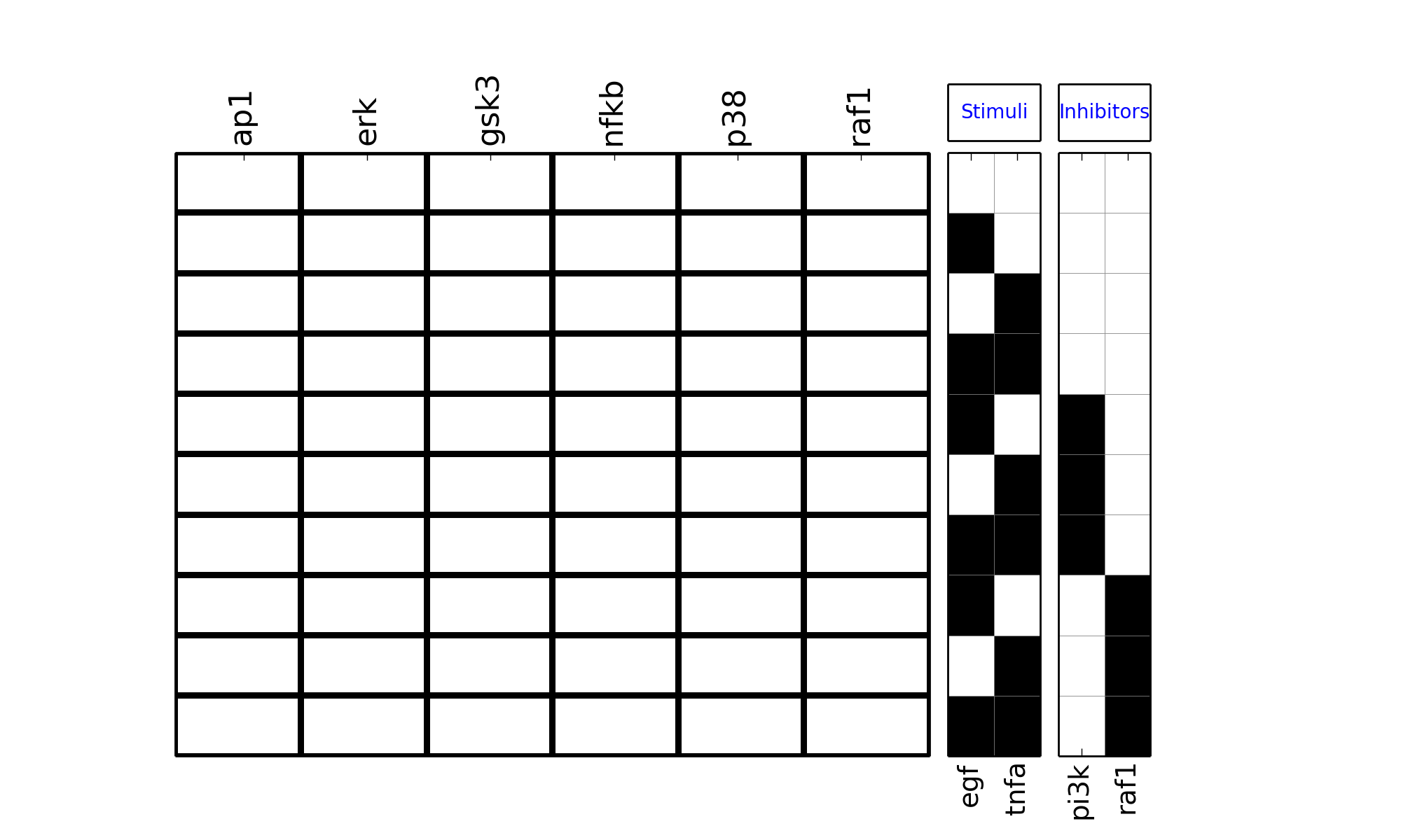
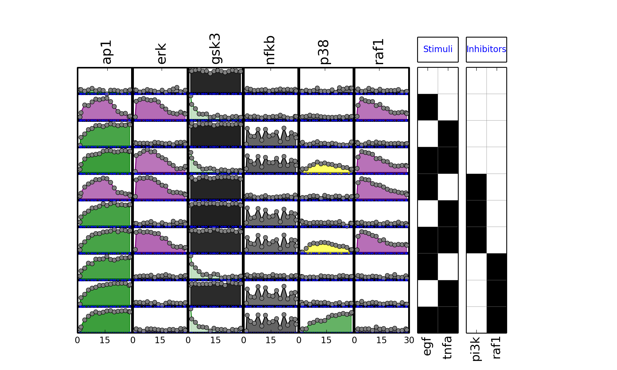
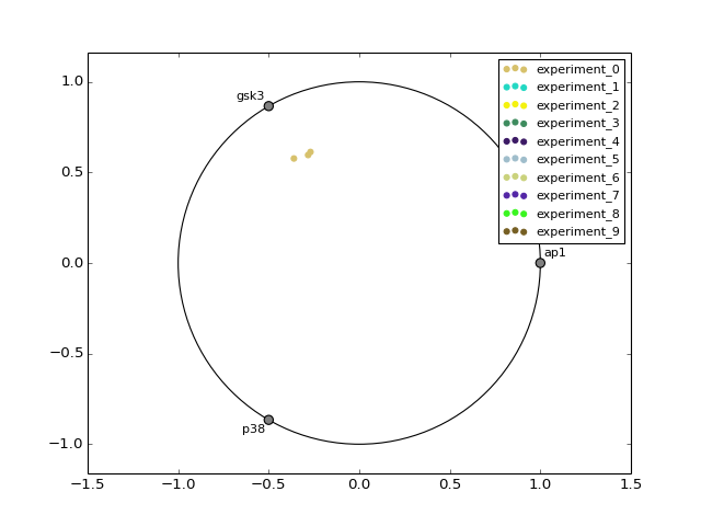
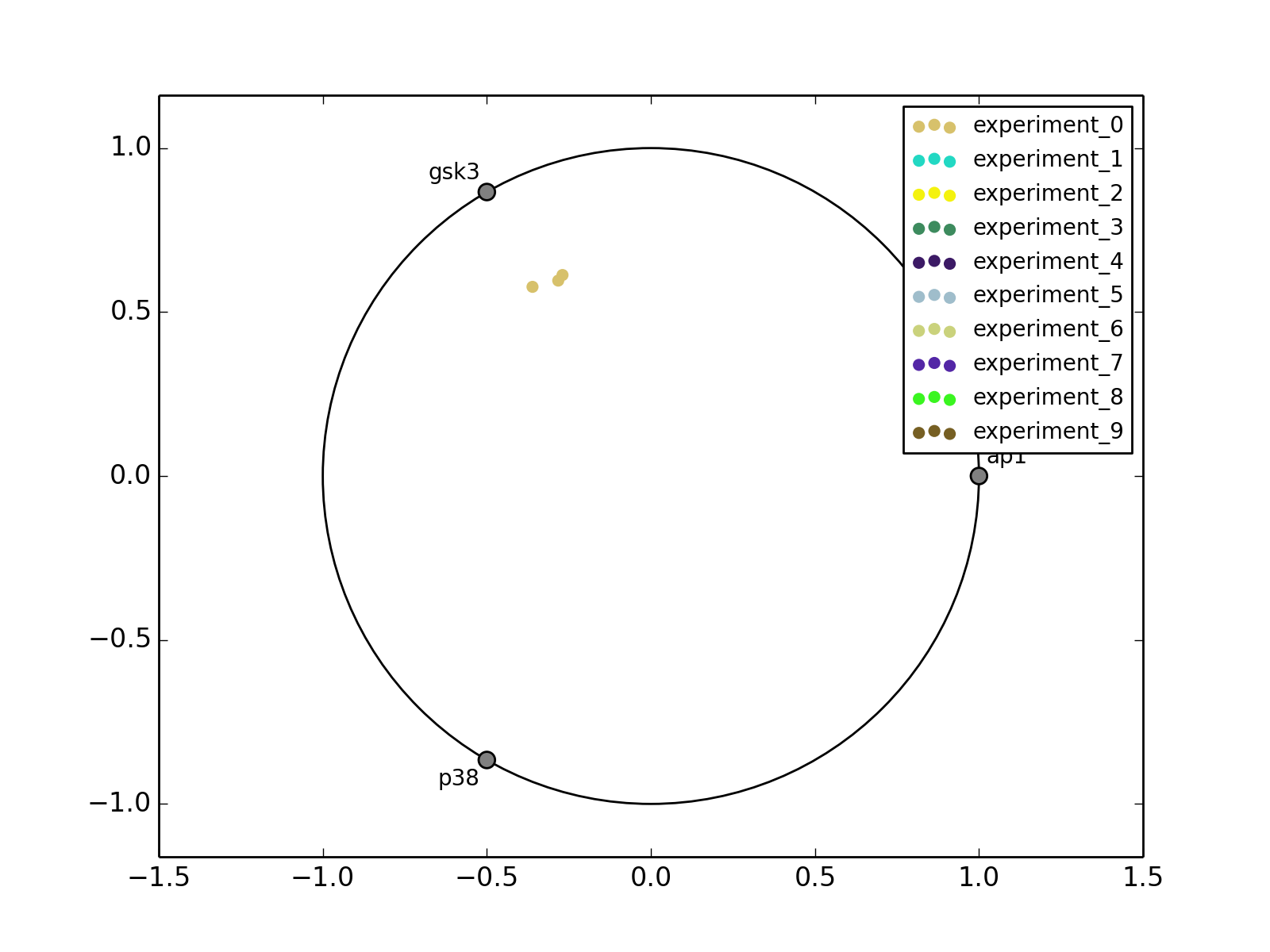
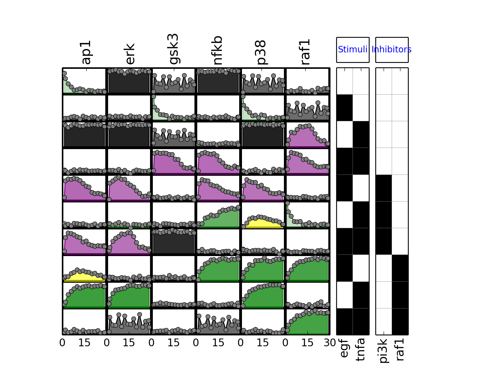
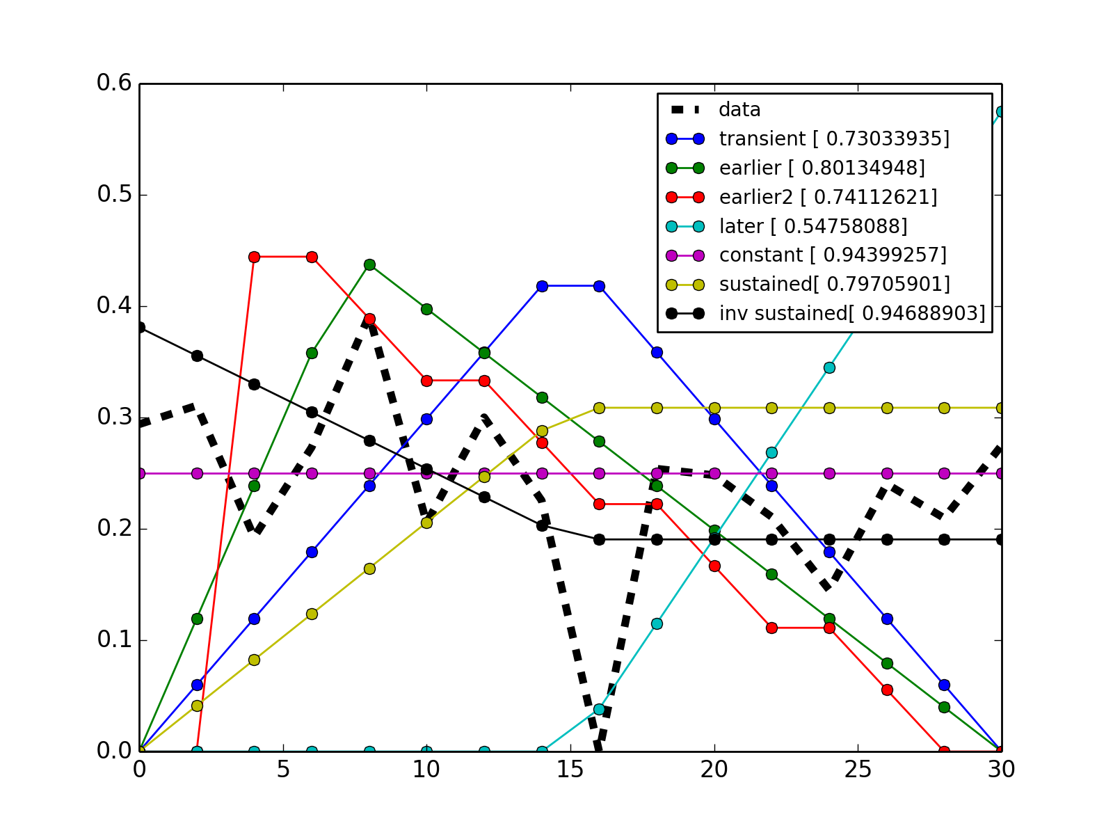
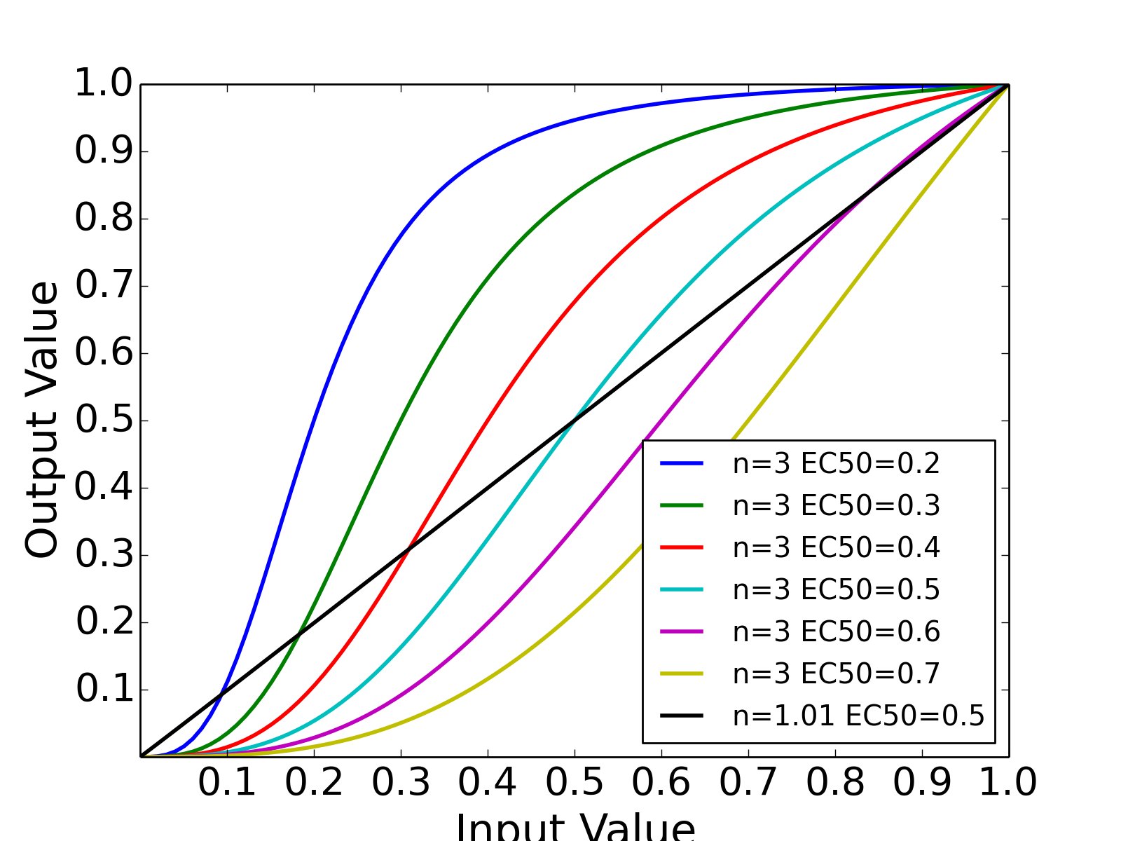
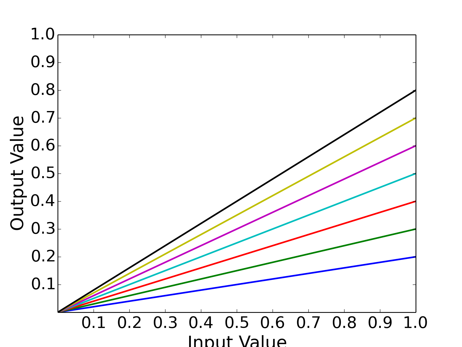
3. For developers
This module provides tools to check out a revision of a SVN directory into a temporary directory and to create a tar ball out of that SVN copy and copy the final tar ball in the directory where this script is called. Sub directories such as .git are removed. The temporary directory is also removed.
This is coded in the DistributeRPackage class. This module is also executable provided with cellnopt.admin package called cellnopt_distribute.
- class DistributeRPackage(package, build_options='--no-build-vignettes')[source]
Class to ease distribution of CellNOptR packages from SVN
Can be used for any SVN containing valid R packages by setting the repository URL
>>> d = DistributeRPackage()
>>> d.distribute()
You can also use the executable provided in cellnopt.admin package itself:
cellnopt_distribute --package CNORdt --revision HEAD
equivalent to (if you have the sources):
python distribute.py --package CNORdt --revision 666
Version of cellnopt.admin were based on private SVN but we moved to github and therefore this class is now related to the github repository only.
In practice, this is more complicated than SVN:
- cannot get a nice revision number and be able to compare between revisions
- Cannot checkout a sub directory (e.g., CNORdt)
So, we will therefore build up all packages in one go and unfortunately add the commit hash long number as a tag....although the –short option seems to be a solution.
Todo
MEIGOR
Parameters: - package (str) – name of a valid package (e.g., CellNOptR)
- revision – SVN revision (default is HEAD )
- build_options – additional build options for R (default is –no-build-vignettes)
You can also change the logging level (e.g., self.logging.debugLevel=”WARNING”)