rabacus.solvers package
Submodules
rabacus.solvers.calc_iliev_sphere module
Solves a sphere with a point source at the center. Canonical examples are Tests 1 and 2 from http://arxiv.org/abs/astro-ph/0603199.
-
class
rabacus.solvers.calc_iliev_sphere.IlievSphere(Edges, T, nH, nHe, rad_src, rec_meth='fixed', fixed_fcA=1.0, atomic_fit_name='hg97', find_Teq=False, z=None, verbose=False, tol=1e-10, thin=False)[source]¶ Stores and calculates equilibrium ionization (and optionally temperature) structure in a spherically symmetric geometry with a point source at the center. The sphere is divided into Nl shells. We will refer to the center of the sphere as “C” and the radius of the sphere as “R”.
- Args:
Edges (array): Radius of all shell edges
T (array): Temperature in each shell
nH (array): Hydrogen number density in each shell
nHe (array): Helium number density in each shell
rad_src (
PointSource): Point source
Note
The arrays T, nH, and nHe must all be the same size. This size determines the number of shells, Nl. Edges determines the positions of the shell edges and must have Nl+1 entries.
Kwargs:
rec_meth (string): How to treat recombinations {“fixed”}
fixed_fcA (float): If rec_meth = “fixed”, constant caseA fraction
atomic_fit_name (string): Source for atomic rate fits {“hg97”}
find_Teq (bool): If
False, use fixed input T, ifTruesolve for equilibrium Tz (float): Redshift, only need if find_Teq =
Trueverbose (bool): Verbose output?
tol (float): tolerance for all convergence tests
thin (bool): if
Trueonly solves optically thinAttributes:
U (
Units)r_c (array): distance from C to center of shell
dr (array): radial thickness of shell
NH_c (array): H column density from C to center of shell
dNH (array): H column density through shell
NH1_c (array): HI column density from C to center of shell
dNH1 (array): HI column density through shell
H1i (array): HI photo-ionization rate
H1h (array): HI photo-heating rate
xH1 (array): H neutral fraction nHI / nH
xH2 (array): H ionized fraction nHII / nH
ne (array): electron number density
fcA_H2 (array): HII case A fraction
cool (array): cooling rate [erg / (cm^3 K)]
heat (array): heating rate [erg / (cm^3 K)]
heatH1 (array): contribution to heat from H1 photo-heating
dtauH1_th (array): HI optical depth at H1 ionizing threshold through shell
tauH1_th_lo (array): HI optical depth below this shell
tauH1_th_hi (array): HI optical depth above this shell
NH1_thru (float): HI column density from C to R
Nl (int): Number of shells
itr (int): Number of iterations to converge
Note
For many of the attributes above, there are analagous versions for helium. We also note that the source of the atomic rates fit is stored in the variable atomic_fit_name, but the source of the photoionization cross section fits are stored in the point source object in the variable px_fit_type.
Examples:
The following code will solve a monochromatic point source inside a spherical distribution with fixed recombination rates and temperatues. In this case we use a Haardt and Madau 2012 spectrum to calculate a grey photon energy which is then used to create a monochromatic plane source
import numpy as np
import rabacus as ra

# create Haardt and Madau 2012 source
#---------------------------------------------------------------
q_min = 1.0; q_max = 4.0e2; z = 3.0
hm12 = ra.rad_src.PointSource( q_min, q_max, 'hm12', z=z )

# get grey photon energy and create a monochromatic plane source
#---------------------------------------------------------------
q_mono = hm12.grey.E.He2 / hm12.PX.Eth_H1
mono = ra.rad_src.PointSource( q_mono, q_mono, 'monochromatic' )
mono.normalize_Ln( 5.0e48 / ra.U.s )

# describe slab
#---------------------------------------------------------------
Nl = 512; Yp = 0.24
nH = np.ones(Nl) * 1.0e-3 / ra.U.cm**3
nHe = nH * Yp * 0.25 / (1.0-Yp)
Tslab = np.ones(Nl) * 1.0e4 * ra.U.K
Rsphere = 6.6 * ra.U.kpc
Edges = np.linspace( 0.0 * ra.U.kpc, Rsphere, Nl+1 )

# solve slab
#---------------------------------------------------------------
sphere = ra.solvers.IlievSphere( Edges, Tslab, nH, nHe, mono,
                                 rec_meth='fixed', fixed_fcA=0.0 )
-
set_optically_thin()[source]¶ Set optically thin ionzation state at input temperature. Adjustments will be made during the sweeps.
rabacus.solvers.calc_slab module
Solves a slab with plane parallel radiation incident from one side.
-
class
rabacus.solvers.calc_slab.Slab(Edges, T, nH, nHe, rad_src, rec_meth='fixed', fixed_fcA=1.0, thresh_P_A=0.01, thresh_P_B=0.99, thresh_xmfp=30.0, atomic_fit_name='hg97', find_Teq=False, z=None, verbose=False, tol=1e-10, thin=False)[source]¶ Solves a slab geometry with plane parallel radiation incident from one side. The slab is divided into Nl layers.
- Args:
Edges (array): Distance to layer edges
T (array): Temperature in each layer
nH (array): hydrogen number density in each layer
nHe (array): helium number density in each layer
rad_src (
PlaneSource): Plane source
Note
The arrays T, nH, and nHe must all be the same size. This size determines the number of shells, Nl. Edges determines the positions of the layer edges and must have Nl+1 entries.
Kwargs:
rec_meth (string): How to treat recombinations {
fixed,thresh}fixed_fcA (float): If rec_meth =
fixed, constant caseA fractionthresh_P_A (float): If rec_meth =
thresh, this is the probability of absorption, P = 1 - exp(-tau), at which the transition to caseB rates begins.thresh_P_B (float): If rec_meth =
thresh, this is the probability of absorption, P = 1 - exp(-tau), at which the transition to caseB ends.thresh_xmfp (float): Determines the distance to probe when calculating optical depth for the caseA to caseB transition. Specifies a multiple of the mean free path for fully neutral gas. In equation form, L = thresh_xmfp / (n * sigma)
atomic_fit_name (string): Source for atomic rate fits {
hg97}find_Teq (bool): If
False, use fixed input T, ifTruesolve for equilibrium Tz (float): Redshift, only need if find_Teq =
Trueverbose (bool): Verbose output?
tol (float): tolerance for all convergence tests
thin (bool): if
Trueonly solves optically thinAttributes:
U (
Units)z_c (array): distance from surface of slab to center of layer
dz (array): thickness of layer
NH_c (array): H column density from surface of slab to center of layer
dNH (array): H column density through layer
NH1_c (array): HI column density from surface of slab to center of layer
dNH1 (array): HI column density through layer
H1i (array): HI photo-ionization rate
H1h (array): HI photo-heating rate
xH1 (array): H neutral fraction nHI / nH
xH2 (array): H ionized fraction nHII / nH
ne (array): electron number density
fcA_H2 (array): HII case A fraction
cool (array): cooling rate [erg / (cm^3 K)]
heat (array): heating rate [erg / (cm^3 K)]
heatH1 (array): contribution to heat from H1 photoheating
dtauH1_th (array): HI optical depth at H1 ionizing threshold through layer
tauH1_th_lo (array): HI optical depth below this layer
tauH1_th_hi (array): HI optical depth above this layer
NH1_thru (float): HI column density through entire slab
Nl (int): Number of layers
itr (int): Number of iterations to converge
Note
For many of the attributes above, there are analagous versions for helium. We also note that the source of the atomic rates fit is stored in the variable atomic_fit_name, but the source of the photoionization cross section fits are stored in the point source object in the variable px_fit_type.
Examples:
The following code will solve a monochromatic source incident onto a slab with fixed recombination rates and temperatues. In this case we use a Haardt and Madau 2012 spectrum to calculate a grey photon energy which is then used to create a monochromatic plane source
import numpy as np
import rabacus as ra

# create Haardt and Madau 2012 source
#---------------------------------------------------------------
q_min = 1.0; q_max = 4.0e2; z = 3.0
hm12 = ra.rad_src.PlaneSource( q_min, q_max, 'hm12', z=z )

# get grey photon energy and create a monochromatic plane source
#---------------------------------------------------------------
q_mono = hm12.grey.E.He2 / hm12.PX.Eth_H1
mono = ra.rad_src.PlaneSource( q_mono, q_mono, 'monochromatic' )
mono.normalize_H1i( hm12.thin.H1i )

# describe slab
#---------------------------------------------------------------
Nl = 512; Yp = 0.24
nH = np.ones(Nl) * 1.5e-2 / ra.U.cm**3
nHe = nH * Yp * 0.25 / (1.0-Yp)
Tslab = np.ones(Nl) * 1.0e4 * ra.U.K
Lslab = 200.0 * ra.U.kpc
Edges = np.linspace( 0.0 * ra.U.kpc, Lslab, Nl+1 )

# solve slab
#---------------------------------------------------------------
slab = ra.solvers.Slab( Edges, Tslab, nH, nHe, mono,
                        rec_meth='fixed', fixed_fcA=1.0 )
-
return_bounds(i, Ltarget)[source]¶ Given a shell number and a distance, return the indices such that self.r[i] - self.r[ii] > Ltarget and self.r[ff] - self.r[i] > Ltarget.
-
return_fcA(tau_th)[source]¶ Given the optical depth at nu_th for any given species, returns the case A fraction.
-
set_fcA(i)[source]¶ Calculate case A fraction for each species in this layer.
- Args:
- i (int): layer index
rabacus.solvers.calc_slab_2 module
Solves a slab with plane parallel radiation incident from both sides.
-
class
rabacus.solvers.calc_slab_2.Slab2(Edges, T, nH, nHe, rad_src, rec_meth='fixed', fixed_fcA=1.0, thresh_P_A=0.01, thresh_P_B=0.99, thresh_xmfp=30.0, atomic_fit_name='hg97', find_Teq=False, z=None, verbose=False, tol=1e-10, thin=False)[source]¶ Solves a slab geometry with plane parallel radiation incident from both sides. The slab is divided into Nl layers.
- Args:
Edges (array): Distance to layer edges
T (array): Temperature in each layer
nH (array): hydrogen number density in each layer
nHe (array): helium number density in each layer
rad_src (
PlaneSource): Plane source
Note
The arrays T, nH, and nHe must all be the same size. This size determines the number of shells, Nl. Edges determines the positions of the layer edges and must have Nl+1 entries.
Kwargs:
rec_meth (string): How to treat recombinations {“fixed”, “thresh”}
fixed_fcA (float): If rec_meth = “fixed”, constant caseA fraction
thresh_P_A (float): If rec_meth = “thresh”, this is the probability of absorption, P = 1 - exp(-tau), at which the transition to caseB rates begins.
thresh_P_B (float): If rec_meth = “thresh”, this is the probability of absorption, P = 1 - exp(-tau), at which the transition to caseB ends.
thresh_xmfp (float): Determines the distance to probe when calculating optical depth for the caseA to caseB transition. Specifies a multiple of the mean free path for fully neutral gas. In equation form, L = thresh_xmfp / (n * sigma)
atomic_fit_name (string): Source for atomic rate fits {“hg97”}
find_Teq (bool): If
False, use fixed input T, ifTruesolve for equilibrium Tz (float): Redshift, only need if find_Teq =
Trueverbose (bool): Verbose output?
tol (float): tolerance for all convergence tests
thin (bool): if
Trueonly solves optically thinAttributes:
U (
Units)z_c (array): distance from surface of slab to center of layer
dz (array): thickness of layer
NH_c (array): H column density from surface of slab to center of layer
dNH (array): H column density through layer
NH1_c (array): HI column density from surface of slab to center of layer
dNH1 (array): HI column density through layer
H1i (array): HI photo-ionization rate
H1h (array): HI photo-heating rate
xH1 (array): H neutral fraction nHI / nH
xH2 (array): H ionized fraction nHII / nH
ne (array): electron number density
fcA_H2 (array): HII case A fraction
cool (array): cooling rate [erg / (cm^3 K)]
heat (array): heating rate [erg / (cm^3 K)]
heatH1 (array): contribution to heat from H1 photoheating
dtauH1_th (array): HI optical depth at H1 ionizing threshold through layer
tauH1_th_lo (array): HI optical depth below this layer
tauH1_th_hi (array): HI optical depth above this layer
NH1_thru (float): HI column density through entire slab
Nl (int): Number of layers
itr (int): Number of iterations to converge
Note
For many of the attributes above, there are analagous versions for helium. We also note that the source of the atomic rates fit is stored in the variable atomic_fit_name, but the source of the photoionization cross section fits are stored in the point source object in the variable px_fit_type.
Examples:
The following code will solve a monochromatic source incident onto a slab with fixed recombination rates and temperatues. In this case we use a Haardt and Madau 2012 spectrum to calculate a grey photon energy which is then used to create a monochromatic plane source
import numpy as np
import rabacus as ra

# create Haardt and Madau 2012 source
#---------------------------------------------------------------
q_min = 1.0; q_max = 4.0e2; z = 3.0
hm12 = ra.rad_src.PlaneSource( q_min, q_max, 'hm12', z=z )

# get grey photon energy and create a monochromatic plane source
#---------------------------------------------------------------
q_mono = hm12.grey.E.He2 / hm12.PX.Eth_H1
mono = ra.rad_src.PlaneSource( q_mono, q_mono, 'monochromatic' )
mono.normalize_H1i( hm12.thin.H1i )

# describe slab
#---------------------------------------------------------------
Nl = 512; Yp = 0.24
nH = np.ones(Nl) * 1.5e-2 / ra.U.cm**3
nHe = nH * Yp * 0.25 / (1.0-Yp)
Tslab = np.ones(Nl) * 1.0e4 * ra.U.K
Lslab = 200.0 * ra.U.kpc
Edges = np.linspace( 0.0 * ra.U.kpc, Lslab, Nl+1 )

# solve slab
#---------------------------------------------------------------
slab = ra.solvers.Slab2( Edges, Tslab, nH, nHe, mono,
                         rec_meth='fixed', fixed_fcA=1.0 )
-
init_slab()[source]¶ Initialize slab values. We will refer to the surface that coincides with layer 0 as Slo and the surface that coincides with layer Nl-1 as Shi.
-
return_bounds(i, Ltarget)[source]¶ Given a shell number and a distance, return the indices such that self.r[i] - self.r[ii] > Ltarget and self.r[ff] - self.r[i] > Ltarget.
-
return_fcA(tau_th)[source]¶ Given the optical depth at nu_th for any given species, returns the case A fraction.
-
set_fcA(i)[source]¶ Calculate case A fraction for each species in this layer.
- Args:
- i (int): layer index
rabacus.solvers.calc_slab_analytic module
Provides an analytic solution for a pure hydrogen constant density and temperature slab with monochromatic plane parallel radiation incident from one side.
-
class
rabacus.solvers.calc_slab_analytic.AnalyticSlab(nH, T, H1i_0, y, fcA, Nsamp=500)[source]¶ Solves an analytic slab. The distance variable used in this solution is the fully neutral optical depth, tauH. To convert this to a distance provide the hydrogen photoionization cross section at a given frequency.
- Args:
nH (float): constant hydrogen number density
T (float); constant temperature
H1i_0 (float): hydrogen photoionization rate at surface of slab
y (float): quantifies electrons from elements heavier than H, ne = nH * (xH2 + y) (throughout slab)
fcA (float) constant case A recombination fraction.
- Kwargs:
- Nsamp (int): number of spatial samples.
rabacus.solvers.one_zone module
Single zone ionization and temperature solvers for primordial gas.
-
class
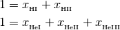
rabacus.solvers.one_zone.Solve_CE(kchem, fpc=True)[source]¶ Calculates and stores collisional ionization equilibrium (i.e. all photoionization rates are equal to zero) given a chemistry rates object. This is an exact analytic solution.
Args:
kchem (ChemistryRates): Chemistry ratesKwargs:
fpc (bool): If True, perform floating point error correction.Attributes:
T (array): temperature
T_floor (float): minimum possible input temperature
H1 (array): neutral hydrogen fraction,
 =
=  /
/ 
H2 (array): ionized hydrogen fraction,
 =
=  /
/ He1 (array): neutral helium fraction,
 =
=  /
/ 
He2 (array): singly ionized helium fraction,
 =
=  /
/ He3 (array): doubly ionized helium fraction,
 =
=  /
/ Notes:
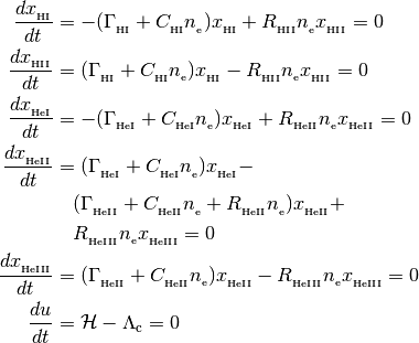
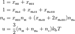
This class finds solutions (H1, H2, He1, He2, He3) to the following equations
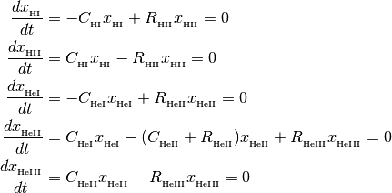
with the following closure relationship
where the
 are collisional ionization rates and the
 are recombination rates. These solutions depend only
on temperature.
are recombination rates. These solutions depend only
on temperature.Examples:
The following code will solve for collisional ionization equilibrium at 128 temperatures equally spaced between 1.0e4 and 1.0e5 K using case A recombination rates for all species:
import numpy as np
import rabacus as ra
N = 128
T = np.logspace( 4.0, 5.0, N ) * ra.u.K
fcA_H2 = 1.0; fcA_He2 = 1.0; fcA_He3 = 1.0
kchem = ra.ChemistryRates( T, fcA_H2, fcA_He2, fcA_He3 )
x_ce = ra.solvers.Solve_CE( kchem )
See also
-
set(kchem)[source]¶ This function is called when a new instance of
Solve_CEis created. Updated ionization fractions can be calculated by calling it again with a new kchem object.Args:
kchem (ChemistryRates): Chemistry rates
-
-
class
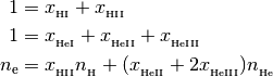
rabacus.solvers.one_zone.Solve_PCE(nH_in, nHe_in, kchem, fpc=True, verbose=False, two_dim_output=False, tol=1e-10)[source]¶ Stores and calculates photo-collisional ionization equilibrium given the density of hydrogen and helium plus a chemistry rates object. This is an iterative solution. The shape of the output depends on the shape of the input arrays. There are two important numbers, Nrho and NT. Nrho is the size of the density arrays nH_in and nHe_in (both of which must be the same). NT is the size of the temperature array in kchem. If two_dim_output =
False, the density and temperature arrays must have the same size and the output arrays are 1-D of that size. If two_dim_output =True, all the main output arrays will have shape (Nrho,NT). In this case, an ionization state solution will be produced for each possible combination of input density and temperature.Note
The user must pass in photoionization rates for each species when creating the chemistry rates object (see examples below).
Args:
nH_in (array): number density of hydrogen
nHe_in (array): number density of helium
kchem (
ChemistryRates): chemistry ratesKwargs:
fpc (bool): If
True, perform floating point error correction.verbose (bool): If
True, produce verbose outputtwo_dim_output (bool): If
True, produce a solution for every possible density-temperature pairtol (float): convergence tolerance, abs(1 - ne_new / ne_old) < tol
Attributes:
nH (array): H number density. Matches output array shape (i.e. equal to nH_in if two_dim_output = False.)
nHe (array): He number density. Matches output array shape. (i.e. equal to nHe_in if two_dim_output = False.)
ne (array): electron number density
T (array): temperature
T_floor (float): minimum possible temperature
H1 (array): neutral hydrogen fraction,
= / H2 (array): ionized hydrogen fraction,
= / He1 (array): neutral helium fraction,
= / He2 (array): singly ionized helium fraction,
= / He3 (array): doubly ionized helium fraction,
= / Hatom (
Hydrogen): H atomitr (int): number of iterations to converge
ne_min (array): electron density in collisional equilibrium
ne_max (array): electron density for full ionization
xH1_ana (array): analytic H neutral fraction (neglects electrons from elements other than H)
ne_ana (array): electron number density implied by xH1_ana
x_ce (
Solve_CE): the collisional equilibrium solutions.Notes:
This class finds solutions (H1, H2, He1, He2, He3) to the following equations
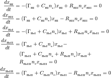
with the following closure relationships
where the
 are photoionization rates, the
are collisional ionization rates and the
are recombination rates. These solutions depend on
temperature and density.
are photoionization rates, the
are collisional ionization rates and the
are recombination rates. These solutions depend on
temperature and density.Examples:
The 1-D output is the default setting. The following code will solve for photo-collisional ionization equilibrium at 128 density-temperature pairs using recombination rates half way between case A and case B for all species. Note that the photoionization rate arrays are grouped with the chemistry rates and so should always be the same size as the temperature array:
import numpy as np
import rabacus as ra

fcA_H2 = 0.5; fcA_He2 = 0.5; fcA_He3 = 0.5

N = 128; Nrho = NT = N; Yp = 0.24

nH = np.linspace( 1.0e-4, 1.0e-3, Nrho ) / ra.U.cm**3
nHe = nH * 0.25 * Yp / (1-Yp)
T = np.linspace( 1.0e4, 1.0e5, NT ) * ra.U.K

H1i = np.ones( NT ) * 8.22e-13 / ra.U.s
He1i = np.ones( NT ) * 4.76e-13 / ra.U.s
He2i = np.ones( NT ) * 3.51e-15 / ra.U.s

kchem = ra.atomic.ChemistryRates( T, fcA_H2, fcA_He2, fcA_He3,
                                  H1i=H1i, He1i=He1i, He2i=He2i )

x_pce_1D = ra.solvers.Solve_PCE( nH, nHe, kchem )
If the two_dim_output keyword is set to True, a solution will be produced for all possible combinations of density and temperature. In the following example, the output arrays will have shape (Nrho,NT):
import numpy as np
import rabacus as ra

fcA_H2 = 0.5; fcA_He2 = 0.5; fcA_He3 = 0.5

Nrho = 128; NT = 32; Yp = 0.24

nH = np.linspace( 1.0e-4, 1.0e-3, Nrho ) / ra.U.cm**3
nHe = nH * 0.25 * Yp / (1-Yp)
T = np.linspace( 1.0e4, 1.0e5, NT ) * ra.U.K

H1i = np.ones( NT ) * 8.22e-13 / ra.U.s
He1i = np.ones( NT ) * 4.76e-13 / ra.U.s
He2i = np.ones( NT ) * 3.51e-15 / ra.U.s

kchem = ra.ChemistryRates( T, fcA_H2, fcA_He2, fcA_He3,
                           H1i=H1i, He1i=He1i, He2i=He2i )

x_pce_2D = ra.solvers.Solve_PCE( nH, nHe, kchem,
                                 two_dim_output=True )
See also
-
set(nH_in, nHe_in, kchem)[source]¶ This function is called when a new instance of
Solve_PCEis created. Updated ionization fractions can be calculated by calling it again with new densities and a new kchem object.Args:
nH_in (array): number density of hydrogen
nHe_in (array): number density of helium
kchem (
ChemistryRates): chemistry rates
-
-
class
rabacus.solvers.one_zone.Solve_PCTE(nH_in, nHe_in, kchem, kcool, z, Hz=None, sd93_logZ=None, fpc=True, verbose=False, tol=1e-10)[source]¶ Stores and calculates photo-collisional-thermal ionization and temperature equilibrium given the density of hydrogen and helium plus chemistry and cooling rate objects. In other words, a self-consistent equilibrium temperature and ionization state will be found for the input density and redshift. This is an iterative solution. All input arrays should be 1-D. Note that the temperature arrays in kchem and kcool will be altered. It is not important which temperatures are used to initialize the objects kchem and kcool. It IS important that you initialize them with photoionization and photoheating rates. Because we are searching for one temperature for each density all input arrays must have the same shape.
Note
The user must pass in photoionization rates for each species when creating the chemistry rates object and photoheating rates for each species when creating the cooling rates object (see examples below).
Args:
nH_in (array): number density of hydrogen
nHe_in (array): number density of helium
kchem (
ChemistryRates): chemistry rateskcool (
CoolingRates): cooling ratesz (float): Redshift. Important for Compton cooling
Kwargs:
Hz (float): Hubble parameter at z if Hubble cooling is desired.
sd93_logZ (float): set to log metallicity (log Z) to use metal cooling in CIE from Sutherland and Dopita 1993
fpc (bool): If
True, perform floating point error correction.verbose (bool): If
True, produce verbose outputtol (float): convergence tolerance, abs(1 - ne_new / ne_old) < tol
Attributes:
nH (array): H number density.
nHe (array): He number density.
ne (array): electron number density
T_floor (float): minimum possible temperature
H1 (array): neutral hydrogen fraction,
= / H2 (array): ionized hydrogen fraction,
= / He1 (array): neutral helium fraction,
= / He2 (array): singly ionized helium fraction,
= / He3 (array): doubly ionized helium fraction,
= / Teq (array): equilibrium temperature
cool (array): cooling rate at final state (should be equal to heat)
heat (array): heating rate at final state (should be equal to cool)
itr (int): number of iterations to converge
Tcmb (float): CMB temperature at input redshift
Notes:
This class finds solutions (H1, H2, He1, He2, He3, Teq) to the following equations
with the following closure relationships
In the equations above, the
are photoionization
rates, the are collisional ionization rates, the
are recombination rates,  is the internal
energy,
is the internal
energy,  is the heating function, and
 is the cooling function. These solutions depend
on temperature and density.
is the cooling function. These solutions depend
on temperature and density.Examples:
The following code will solve for photo-collisional-thermal ionization equilibrium at 128 densities using case B recombination rates for all species. The photoionization and heating rates are taken from the Haardt and Madau 2012 model. Note that the photoionization rate arrays are grouped with the chemistry rates and the photo-heating rate arrays are grouped with the cooling rates:
import numpy as np
import rabacus as ra

N = 128; Yp = 0.24; z=3.0
fcA_H2 = fcA_He2 = fcA_He3 = 0.0

nH = np.linspace( 1.0e-4, 1.0e-3, N ) / ra.U.cm**3
nHe = nH * 0.25 * Yp / (1-Yp)
T = np.linspace( 1.0e4, 1.0e5, N ) * ra.U.K

hmr = ra.uv_bgnd.HM12_Photorates_Table()

H1i = np.ones(N) * hmr.H1i(z)
He1i = np.ones(N) * hmr.He1i(z)
He2i = np.ones(N) * hmr.He2i(z)
kchem = ra.atomic.ChemistryRates( T, fcA_H2, fcA_He2, fcA_He3,
                                  H1i=H1i, He1i=He1i, He2i=He2i )

H1h = np.ones(N) * hmr.H1h(z)
He1h = np.ones(N) * hmr.He1h(z)
He2h = np.ones(N) * hmr.He2h(z)
kcool = ra.atomic.CoolingRates( T, fcA_H2, fcA_He2, fcA_He3,
                                H1h=H1h, He1h=He1h, He2h=He2h )

x_pcte = ra.solvers.Solve_PCTE( nH, nHe, kchem, kcool, z )
-
set(nH_in, nHe_in, kchem, kcool, z)[source]¶ This function is called when a new instance of
Solve_PCTEis created. Updated solutions can be calculated by calling it again with new densities and new chemistry and cooling objects.Args:
nH_in (array): number density of hydrogen
nHe_in (array): number density of helium
kchem (
ChemistryRates): chemistry rateskcool (
CoolingRates): cooling ratesz (float): Redshift. Important for Compton and Bremsstrahlung cooling
-
Module contents
Tools for calculating the ionization and temperature structure in primordial
(i.e. composed of only hydrogen and helium) cosmological gas.
The single zone solvers in one_zone form
the core of this package and contain classes for solving three types of
ionization/temperature equilibrium,
- (
Solve_CE) collisional equilibrium in which ionization fractions are found such that collisional ionizations are balanced by recombinations at a fixed temperature. - (
Solve_PCE) photo-collisional equilibrium in which ionization fractions are found such that photo and collisional ionizations are balanced by recombinations at a fixed temperature. - (
Solve_PCTE) photo-collisional-thermal equilibrium in which ionization fractions are found such that photo and collisional ionizations are balanced by recombinations and a temperature is found such that heating balances cooling.
The other modules in this package make use of
one_zone to calculate the ionization
and/or temperature structure in the case of specific geometries and sources.
- (
calc_slab) An infinite plane gas distribution with plane parallel radiation incident from one side. - (
calc_slab_2) An infinite plane gas distribution with plane parallel radiation incident from both sides. - (
calc_iliev_sphere) A spherically symmetric gas distribution with a point source at the center.
Recombination radiation
Recombination radiation is handled in all solutions using the “variable on-the-spot” approximation. In the standard “on-the-spot” approximation, the effect of ionizing recombination photons are modeled by reducing the recombination rate. The recombination rate to all atomic levels is called the case A rate. Recombinations to the ground state can cause ionizations and so a case B rate is defined that negelects these recombinations,

We define a variable called the case A fraction,  , for each
recombining ionic species
, for each
recombining ionic species
 such that the recombination rate used in the solution is,

The solutions above discretize spheres into thin shells and planes into thin
slabs. We will refer to both of these as discrete elements. The main
variable that determines what will be in each discrete
element is rec_meth.
If rec_meth = fixed then a constant case A fraction,
= fixed_fcA, is used in each element. If rec_meth =
thresh, the case A fraction will vary in each discrete element.
For each element, the optical depth is probed out to a fixed
distance,  . The probability of a recombination photon being absorbed
is then calculated,
. The probability of a recombination photon being absorbed
is then calculated,
![P = 1 - \exp[ -\tau(\nu_{\rm _X})]](_images/math/f1c71aae94e83924054417da67e5cad8c869cc29.png)
where  is the optical depth for a given species at
its ionization threshold. This probability is then used to interpolate
between case A and case B rates. The variable
thresh_P_A (
is the optical depth for a given species at
its ionization threshold. This probability is then used to interpolate
between case A and case B rates. The variable
thresh_P_A ( ) determines the probability at which the
transition to case B starts and the variable thresh_P_B (
) determines the probability at which the
transition to case B starts and the variable thresh_P_B ( )
determines the probability at which the transition to case B ends.
The variable thresh_xmfp (
)
determines the probability at which the transition to case B ends.
The variable thresh_xmfp ( ) determines the distance
and represents a multiplier to the fully neutral mean free path in a
discrete element,
) determines the distance
and represents a multiplier to the fully neutral mean free path in a
discrete element,
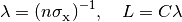
where  is either or .
If
is either or .
If  then
then  ,
if
,
if  then
then  ,
otherwise,
,
otherwise,
