Stromgren Sphere Examples
In this section we will go thourgh some concrete examples using
SphereStromgren.
This class models a spherically symmetric gas distribution with a point source
at the center. In particular we will examine Tests 1 and 2 in the Cosmological
Radiative Transfer Comparison Project (CRTCP) [Iliev06], the work of
[Friedrich12] which includes helium, and the work of [Raicevic14] which
includes radiative transfer of recombination radiation.
Preparation
Import Packages
The following examples require three python packages to be imported,
import numpy as np
import pylab as plt
import rabacus as ra
Plotting Functions
We will be making several plots during the course of these examples. In order to facilitate this, we will define a few convenience functions here,
def plot_sphere_x( s, fname, style, plot_H=True, plot_He=True ):
  """ put plot of ionization fractions from sphere `s` into fname """

  plt.figure( figsize=(7,7) )

  s.r_c.units = 'kpc'
  s.Edges.units = 'kpc'
  if style == 'I':
      xx = s.r_c / s.Edges[-1]
  else:
      xx = s.r_c

  if plot_He:
      plt.plot( xx, np.log10( s.xHe1 ),
                color='green', ls='-', label = r'$x_{\rm HeI}$' )
      plt.plot( xx, np.log10( s.xHe2 ),
                color='green', ls='--', label = r'$x_{\rm HeII}$' )
      plt.plot( xx, np.log10( s.xHe3 ),
                color='green', ls=':', label = r'$x_{\rm HeIII}$' )

  if plot_H:
      plt.plot( xx, np.log10( s.xH1 ),
                color='red', ls='-', label = r'$x_{\rm HI}$' )
      plt.plot( xx, np.log10( s.xH2 ),
                color='red', ls='--', label = r'$x_{\rm HII}$' )

  if style == 'I':
      plt.xlim( -0.05, 1.05 )
      plt.xlabel( 'r_c / Rsphere' )
  else:
      plt.xlim( -0.50, 15.2 )
      plt.xlabel( 'r_c [kpc]' )

  if style == 'I':
      plt.ylim( -6.0, 0.5 )
  else:
      plt.ylim( -3.1, 0.1 )
  plt.ylabel( 'log 10 ( x )' )

  plt.grid()
  plt.legend(loc='lower center', ncol=2)
  plt.tight_layout()
  plt.savefig( 'doc/img/x' + fname )


def plot_sphere_T( s, fname, style ):
  """ put plot of temperature from sphere `s` into fname """

  plt.figure( figsize=(7,7) )

  s.r_c.units = 'kpc'
  s.Edges.units = 'kpc'
  if style == 'I':
      xx = s.r_c / s.Edges[-1]
  else:
      xx = s.r_c

  plt.plot( xx, s.T,
            color='black', ls='-', label = r'$T$' )

  if style == 'I':
      plt.xlim( -0.05, 1.05 )
      plt.xlabel( 'r_c / Rsphere' )
  else:
      plt.xlim( -0.50, 15.2 )
      plt.xlabel( 'r_c [kpc]' )

  plt.ylim( 0.0, 5.0e4 )
  plt.ylabel( 'T [K]' )

  plt.grid()
  plt.legend(loc='best')
  plt.tight_layout()
  plt.savefig( 'doc/img/T_' + fname )
Create Sources
Next we will setup three point sources, one monochromatic, one with a thermal spectrum, and one with a powerlaw spectrum. We will normalize all spectra such that they emit the same number of photons per second,
Ln = 5.0e48 / ra.u.s  # set photon luminosity

q_mono = 1.0
q_min = q_mono
q_max = q_mono
src_mono = ra.PointSource( q_min, q_max, 'monochromatic' )
src_mono.normalize_Ln( Ln )

q_min = 1.0
q_max = 10.0
T_eff = 1.0e5 * ra.u.K
src_thrm = ra.PointSource( q_min, q_max, 'thermal', T_eff=T_eff )
src_thrm.normalize_Ln( Ln )

q_min = 1.0
q_max = 10.0
alpha = -1.0
src_pwr1 = ra.PointSource( q_min, q_max, 'powerlaw', alpha=alpha )
src_pwr1.normalize_Ln( Ln )
Iliev06 Examples
Setup
To begin, we define a sphere as descibed in [Iliev06]. Note that we take the helium density from [Friedrich12] and also define a null helium densiy which is much lower in order to approximate a zero helium environment.
Nl = 512
T = np.ones(Nl) * 1.0e4 * ra.u.K

Rsphere = 6.6 * ra.u.kpc
Edges = np.linspace( 0.0 * ra.u.kpc, Rsphere, Nl+1 )
nH = np.ones(Nl) * 1.0e-3 / ra.u.cm**3
nHe = np.ones(Nl) * 8.7e-5 / ra.u.cm**3
nHe_null = np.ones(Nl) * 1.0e-15 / ra.u.cm**3
Optically Thin
We begin with a very basic scenario, a pure hydrogen sphere with constant
density and temperature. We place a monochromatic source at the center
but allow only geometric dillution of the radiation by setting the keyword
thin to True. By default, case A recombination rates are used. We use
case B recombination rates by setting the keyword fixed_fcA to 0.0.
key = 'thin_caseB_mono_fixT'

spheres[key] = ra.SphereStromgren(
    Edges, T, nH, nHe_null, src_mono, fixed_fcA=0.0, thin=True )

plot_sphere_x(
    spheres[key], 'strm_sphere_' + key + '.png', 'I', plot_He=False )

Stromgren Sphere - Thin - Case B - Mono - Fixed T
In this case, the gas remains ionized at all radii.
Test 1
Test 1 of [Iliev06] also involves a pure hydrogen sphere with constant density and temperature and a central monochromatic source. We call the solver with the same input except this time we leave out the keyword thin so the radiation will be attenuated by the gas. The resulting figure can be compared directly to the right panel of Fig. 8 in [Iliev06] (reproduced below).
key = 'rt_caseB_mono_fixT'

spheres[key] = ra.SphereStromgren(
    Edges, T, nH, nHe_null, src_mono, fixed_fcA=0.0 )

plot_sphere_x(
    spheres[key], 'strm_sphere_' + key + '.png', 'I', plot_He=False )
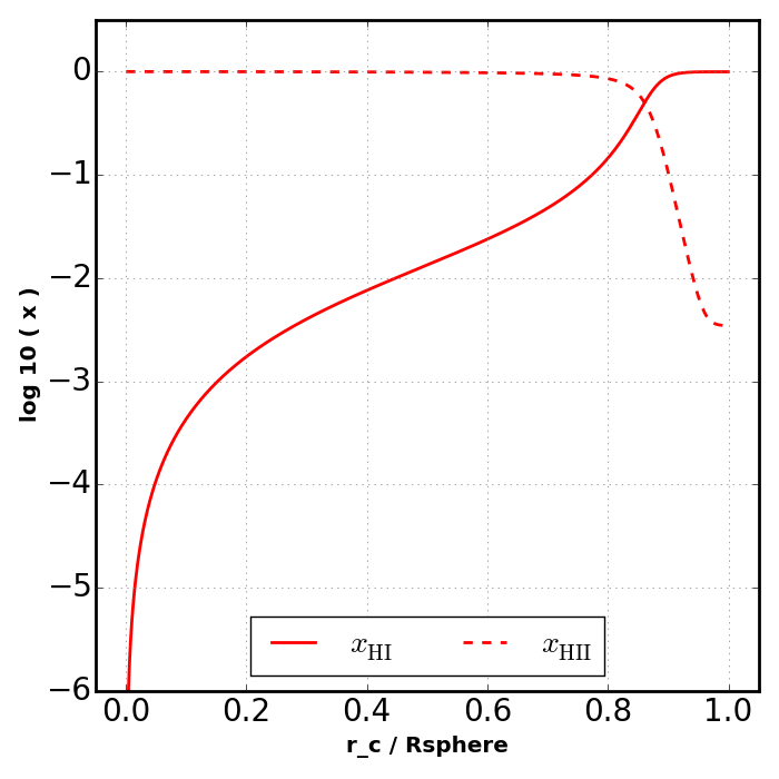
Stromgren Sphere - RT - Case B - Mono - Fixed T
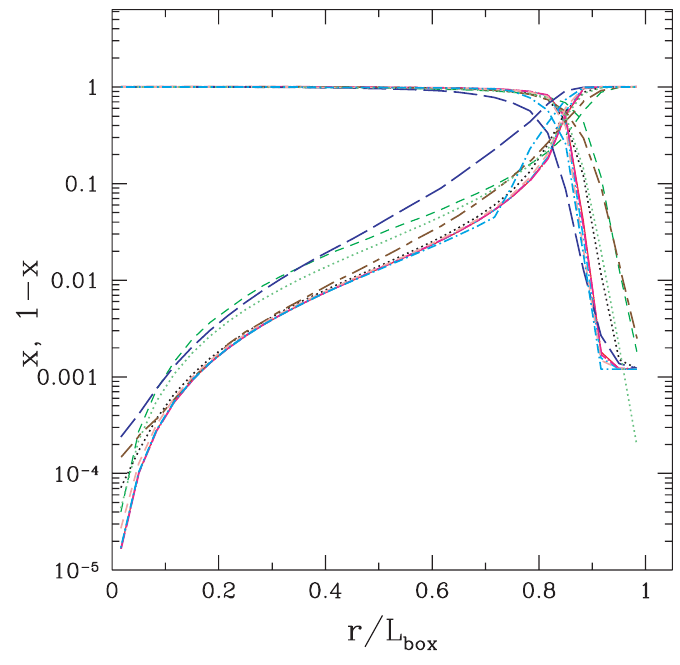
[Iliev06] - Fig. 8
Test 2
Test 2 of [Iliev06] uses a 1.0e5 K thermal spectrum and allows the gas
temperature to vary. We model this situation by setting the find_Teq
keyword to True and passing in src_thrm instead of src_mono.
Note that when find_Teq is True we also have to pass in
a redshift using the keyword z so that Compton cooling can be accounted
for. These figures can be compared directly to the rightmost panels of Figs.
16 and 17 in [Iliev06] (reproduced below).
key = 'rt_caseB_thrm_evoT'

spheres[key] = ra.SphereStromgren(
    Edges, T, nH, nHe_null, src_thrm, fixed_fcA=0.0, find_Teq=True, z=0.0 )

plot_sphere_x(
    spheres[key], 'strm_sphere_' + key + '.png', 'I', plot_He=False )
plot_sphere_T(
    spheres[key], 'strm_sphere_' + key + '.png', 'I' )

Stromgren Sphere - RT - Case B - Thermal - Equilibrium T
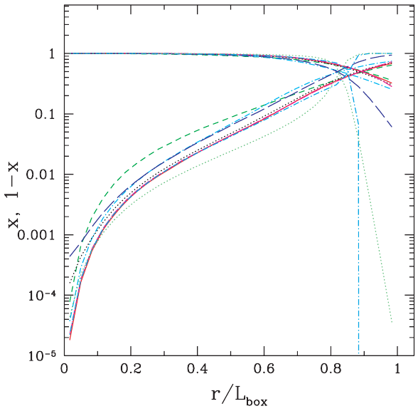
[Iliev06] - Fig. 16
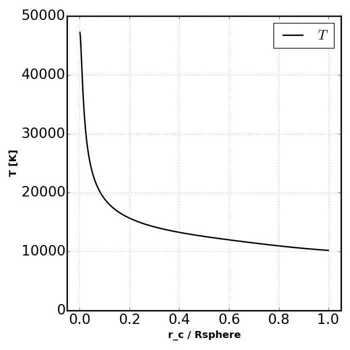
Iliev Sphere - RT - Case B - Thermal - Equilibrium T
[Iliev06] - Fig. 17
Friedrich12 Examples
We now focus on the tests presented in [Friedrich12]. They are based on those described in [Iliev06] except they include helium. Because of the longer mean free path of helium ionizing photons, the radius of the sphere is increased to 15 kpc.
Rsphere = 15.0 * ra.u.kpc
Edges = np.linspace( 0.0 * ra.u.kpc, Rsphere, Nl+1 )
Test 1 A
Test 1 A, examines a fixed temperature sphere, uses a thermal spectrum, and case A recombination rates. The Rabacus figure can be compared to the panels in Fig. 4 of [Friedrich12] (reproduced below). Because Rabacus produces equilibrium solutions, the lines in this figure should technically be compared to the CLOUDY results in [Friedrich12].
key = 'rt_caseA_thrm_fixT'

spheres[key] = ra.SphereStromgren(
    Edges, T, nH, nHe, src_thrm, fixed_fcA=1.0 )

plot_sphere_x( spheres[key], 'strm_sphere_' + key + '.png', 'F' )
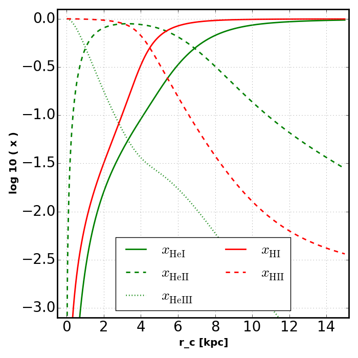
Stromgren Sphere - RT - Case A - Thermal - Fixed T
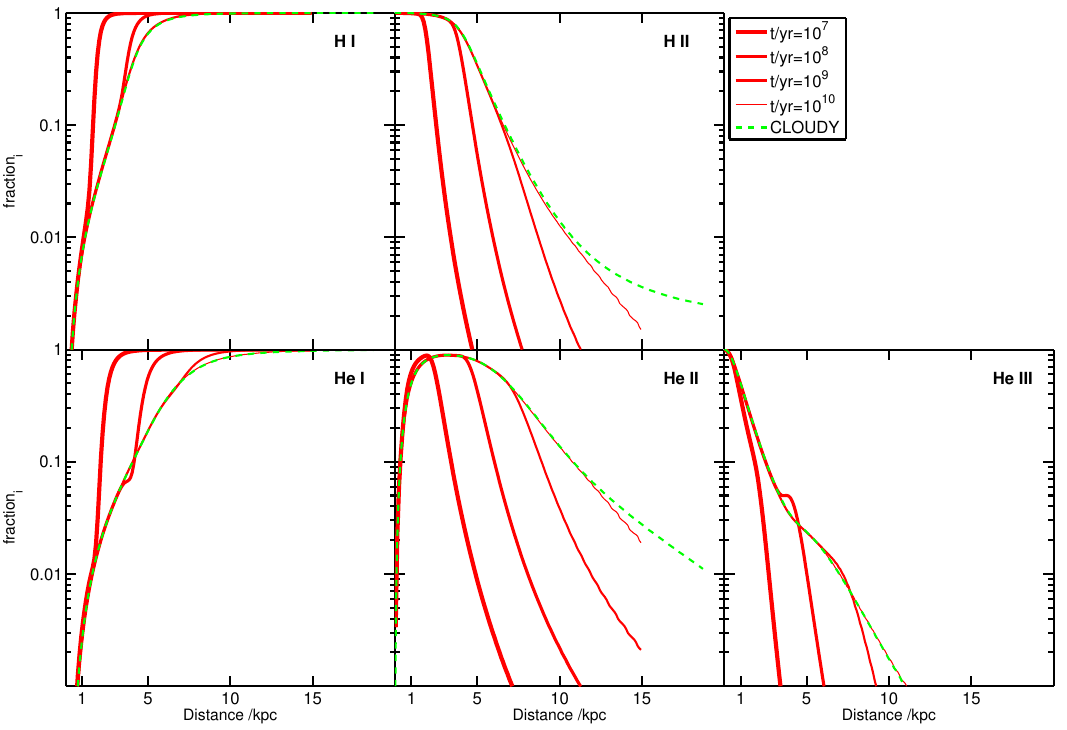
[Friedrich12] - Fig. 4
Note
The maximum energy of photons considered when constructing the spectra
in [Friedrich12] is unclear. We have used q_max = 10, however
this choice can have order of magnitude effects on the ionization
fractions. For example, try the powerlaw example with q_max = 60
instead of 10 and plot the results.
Test 1 B
Test 1 B, examines a fixed temperature sphere, uses a thermal spectrum, and case B recombination rates (i.e. the on-the-spot approximation). We note that using a case B rate for all ionic species is equivalent to what [Friedrich12] term the U-OTS or the uncoupled on-the-spot approximation. This figure can be compared to the panels in Fig. 5 of [Friedrich12] (reproduced below). Again our equilibrium solutions should technically be compared to the CLOUDY OTS solutions in that plot.
key = 'rt_caseB_thrm_fixT'

spheres[key] = ra.SphereStromgren(
    Edges, T, nH, nHe, src_thrm, fixed_fcA=0.0 )

plot_sphere_x( spheres[key], 'strm_sphere_' + key + '.png', 'F' )

Stromgren Sphere - RT - Case B - Thermal - Fixed T

[Friedrich12] - Fig. 5
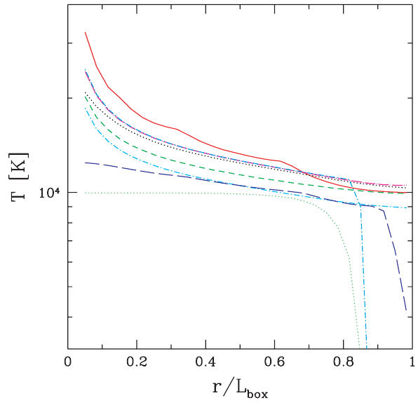
Test 2
Test 2 in [Friedrich12] allows the temperature to vary and examines ionization
profiles in the case of powerlaw sources. They present results for spectra
with powerlaw indices of  and
and  . Here we will
only reproduce the solution. This figure can be compared to
the panels in Fig. 6 of [Friedrich12] (reproduced below). Our equilibrium
solutions should technically be compared to the CLOUDY OTS solutions in that
plot. The dependence on the maximum photon energy included in the spectrum
q_max is stronger for the powerlaw source than for the thermal source.
. Here we will
only reproduce the solution. This figure can be compared to
the panels in Fig. 6 of [Friedrich12] (reproduced below). Our equilibrium
solutions should technically be compared to the CLOUDY OTS solutions in that
plot. The dependence on the maximum photon energy included in the spectrum
q_max is stronger for the powerlaw source than for the thermal source.
key = 'rt_caseB_pwr1_evoT'

spheres[key] = ra.SphereStromgren(
    Edges, T, nH, nHe, src_pwr1, fixed_fcA=0.0, find_Teq=True, z=0.0 )

plot_sphere_x( spheres[key], 'strm_sphere_' + key + '.png', 'F' )
plot_sphere_T( spheres[key], 'strm_sphere_' + key + '.png', 'F' )

Stromgren Sphere - RT - Case B - Powerlaw - Equilibrium T
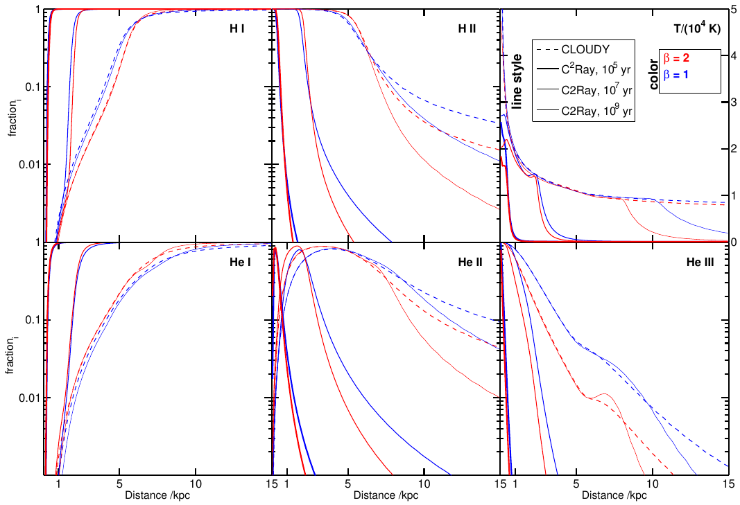
[Friedrich12] - Fig. 6
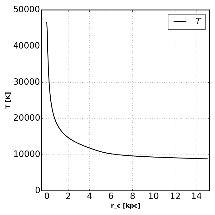
Stromgren Sphere - RT - Case B - Powerlaw - Equilibrium T
Raicevic14 Examples
Now we focus on the treatment of recombination radiation. [Raicevic14] present the results of treating this radiation explicitly using a 3-D radiative transfer code. We will solve the problem by transporting this radiation in our 1-D geometries. First we resize the sphere back to the original CRTCP size,
Rsphere = 6.6 * ra.u.kpc
Edges = np.linspace( 0.0 * ra.u.kpc, Rsphere, Nl+1 )
Recombination Radiation
The first test involves a simple comparison between using fixed case A rates, fixed case B rates, or following the recombination radiation explicitly. We do not have a fixed case A sphere yet so we solve that first,
key = 'rt_caseA_mono_fixT'
spheres[key] = ra.SphereStromgren(
    Edges, T, nH, nHe_null, src_mono, fixed_fcA=1.0 )
Rabacus has three options for the treatment of recombination radiation. In the
first, all recombination radiation is assumed to be transported radially
outward. This makes the assumption that the ionized center of the sphere
produces zero optical depth. This option can be activated by setting the
keyword rec_meth to outward.
key = 'rt_outward_mono_fixT'
spheres[key] = ra.SphereStromgren(
    Edges, T, nH, nHe_null, src_mono, rec_meth='outward' )
The second option transports recombination radiation along radial lines as
well, but accounts for the optical depth encounterd by inward travelling
radiation. This option can be activated by setting the keyword rec_meth
to radial.
key = 'rt_radial_mono_fixT'
spheres[key] = ra.SphereStromgren(
    Edges, T, nH, nHe_null, src_mono, rec_meth='radial' )
The third and most realistic option transports recombination radiation
isotropically from each layer. This option can be activated by setting the
keyword rec_meth to isotropic.
key = 'rt_isotropic_mono_fixT'
spheres[key] = ra.SphereStromgren(
    Edges, T, nH, nHe_null, src_mono, rec_meth='isotropic' )
Below we produce a plot that can be compared to the upper right panel in Fig. 2 of [Raicevic14] (reproduced below).
plt.figure( figsize=(7,7) )

key = 'rt_caseA_mono_fixT'
s = spheres[key]
s.r_c.units = 'kpc'
s.Edges.units = 'kpc'
xx = s.r_c / s.Edges[-1]

key = 'rt_caseA_mono_fixT'
s = spheres[key]
plt.plot( xx, np.log10( s.xH1 ),
          color='blue', ls=':', label = r'case A' )

key = 'rt_caseB_mono_fixT'
s = spheres[key]
plt.plot( xx, np.log10( s.xH1 ),
          color='black', ls='--', label = r'case B' )

key = 'rt_outward_mono_fixT'
s = spheres[key]
plt.plot( xx, np.log10( s.xH1 ),
          color='cyan', ls='-', label = r'outward' )

key = 'rt_radial_mono_fixT'
s = spheres[key]
plt.plot( xx, np.log10( s.xH1 ),
          color='green', ls='-', label = r'radial' )

key = 'rt_isotropic_mono_fixT'
s = spheres[key]
plt.plot( xx, np.log10( s.xH1 ),
          color='red', ls='-', label = r'isotropic' )

plt.xlim( -0.05, 1.05 )
plt.xlabel( 'r_c / Rsphere' )

plt.ylim( -6.0, 0.5 )
plt.ylabel( 'log 10 ( x )' )

plt.grid()
plt.legend(loc='best', ncol=2)
plt.tight_layout()
plt.savefig( 'doc/img/x_raicevic.png' )
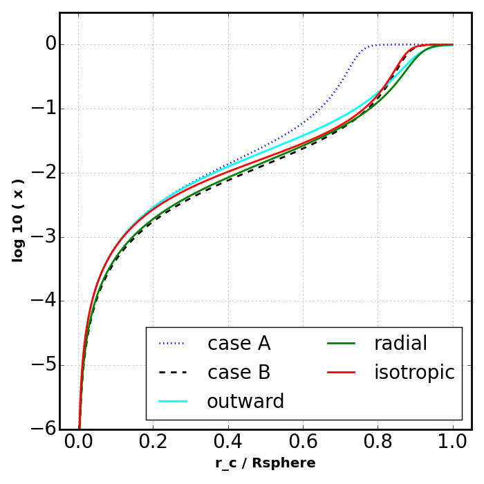
Stromgren Sphere - RT - Case A vs Case B vs Transport
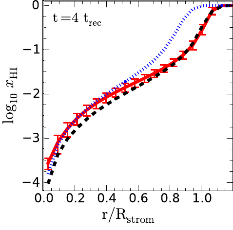
[Raicevic14] - Fig. 2
The outward and radial options produce similar results and
isotropic is the same as [Raicevic14].
Diffuse vs. Source
In the next Figure we show the radiation intensity from the central point
source (source) compared to that from recombinations (diffuse). The
photoionization rates due to the central point source and the diffuse
recombinations are both stored in the returned solved object. The following
plots can be compared to the lower right panel in Fig. 2 of [Raicevic14]
(reproduced below). Here we show the results of using the isotropic
keyword. Note that the x-axis is scaled by the stromgren radius = 5.4 kpc and
not the box length.
plt.figure( figsize=(7,7) )

key = 'rt_isotropic_mono_fixT'
s = spheres[key]
s.r_c.units = 'kpc'
s.Edges.units = 'kpc'
xx = s.r_c / (5.4*ra.u.kpc) # s.Edges[-1]

geo = 4.0 * np.pi * s.r_c**2
I0 = s.H1i_src[0] * geo[0]

# source I/I0
#------------------------------------
Is = s.H1i_src * geo
yy = Is / I0
plt.plot( xx, yy,
          color='red', ls='-', label='source' )

# recomb I/I0
#------------------------------------
Id = s.H1i_rec * geo
yy = Id / I0
plt.plot( xx, yy,
          color='red', ls='--', label='diffuse' )

# ratio diffuse/source
#------------------------------------
yy = Id / Is
plt.plot( xx, yy,
          color='red', ls=':', label='ratio' )

plt.ylabel( r'$I/I_0$', fontsize=25 )
plt.ylim( 0.0, 1.05 )

plt.xlabel( 'r_c / R_strom' )
plt.xlim( -0.05, 1.05 )

plt.grid()
plt.legend(loc='best', ncol=1)
plt.tight_layout()
plt.savefig( 'doc/img/I_raicevic_isotropic.png' )
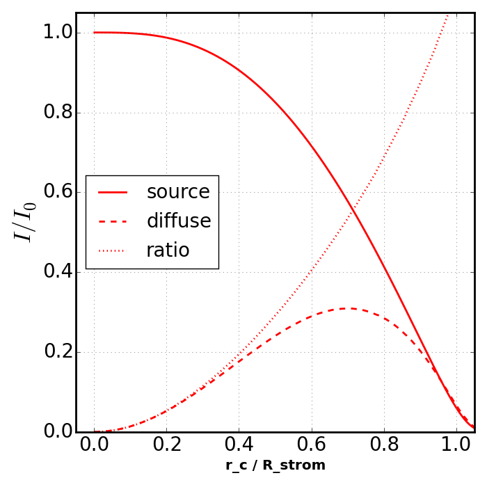
Stromgren Sphere - Source vs Diffuse photons - Isotropic
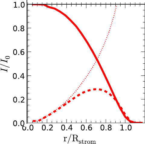
[Raicevic14] - Fig. 2
Making this plot using the sphere solved with the radial model, exposes
the differences between isotropic (and also outward) and radial.
While the results are similar for all three models at large radii, the diffuse
radiation makes a larger contribution at smaller radii in radial. This is
due to the fact that the radial method considers the opacity encountered
by inward travelling recombination radiation.
plt.figure( figsize=(7,7) )

key = 'rt_radial_mono_fixT'
s = spheres[key]
s.r_c.units = 'kpc'
s.Edges.units = 'kpc'
xx = s.r_c / (5.4*ra.u.kpc) # s.Edges[-1]

geo = 4.0 * np.pi * s.r_c**2
I0 = s.H1i_src[0] * geo[0]

# source I/I0
#------------------------------------
Is = s.H1i_src * geo
yy = Is / I0
plt.plot( xx, yy,
          color='green', ls='-', label='source' )

# recomb I/I0
#------------------------------------
Id = s.H1i_rec * geo
yy = Id / I0
plt.plot( xx, yy,
          color='green', ls='--', label='diffuse' )

# ratio diffuse/source
#------------------------------------
yy = Id / Is
plt.plot( xx, yy,
          color='green', ls=':', label='ratio' )

plt.ylabel( r'$I/I_0$', fontsize=25 )
plt.ylim( 0.0, 1.05 )

plt.xlabel( 'r_c / R_strom' )
plt.xlim( -0.05, 1.05 )

plt.grid()
plt.legend(loc='best', ncol=1)
plt.tight_layout()
plt.savefig( 'doc/img/I_raicevic_radial.png' )

Stromgren Sphere - Source vs Diffuse photons - Radial