Background Sphere Examples
In this section we will go thourgh some concrete examples using
SphereBgnd.
This class models a spherically symmetric gas distribution in a uniform
background.
Preparation
Import Packages
The following examples require three python packages to be imported,
import numpy as np
import pylab as plt
import rabacus as ra
Plotting Functions
We will be making several plots during the course of these examples. In order to facilitate this, we will define a few convenience functions here,
def plot_sphere_x( s, fname ):
  """ put plot of ionization fractions from sphere `s` into fname """

  plt.figure()
  s.Edges.units = 'kpc'
  s.r_c.units = 'kpc'
  xx = s.r_c
  L = s.Edges[-1]

  plt.plot( xx, np.log10( s.xHe1 ),
            color='green', ls='-', label = r'$x_{\rm HeI}$' )
  plt.plot( xx, np.log10( s.xHe2 ),
            color='green', ls='--', label = r'$x_{\rm HeII}$' )
  plt.plot( xx, np.log10( s.xHe3 ),
            color='green', ls=':', label = r'$x_{\rm HeIII}$' )

  plt.plot( xx, np.log10( s.xH1 ),
            color='red', ls='-', label = r'$x_{\rm HI}$' )
  plt.plot( xx, np.log10( s.xH2 ),
            color='red', ls='--', label = r'$x_{\rm HII}$' )

  plt.xlim( -L/20, L+L/20 )
  plt.xlabel( 'r_c [kpc]' )

  plt.ylim( -4.5, 0.2 )
  plt.ylabel( 'log 10 ( x )' )

  plt.grid()
  plt.legend(loc='best', ncol=2)
  plt.tight_layout()
  plt.savefig( 'doc/img/x_' + fname )


def plot_sphere_T( s, fname, style ):
  """ put plot of temperature from sphere `s` into fname """

  plt.figure()
  s.Edges.units = 'kpc'
  s.r_c.units = 'kpc'
  xx = s.r_c
  L = s.Edges[-1]

  plt.plot( xx, s.T,
            color='black', ls='-', label = r'$T$' )

  plt.xlim( -L/20, L+L/20 )
  plt.xlabel( 'r_c [kpc]' )

  plt.ylim( 0.0, 3.0e4 )
  plt.ylabel( 'T [K]' )

  plt.grid()
  plt.legend(loc='best')
  plt.tight_layout()
  plt.savefig( 'doc/img/T_' + fname )
Create Sources
Next we will setup two background sources, one monochromatic, and one with the spectrum from the model of Haardt and Madau 2012 [HM12]. We will normalize the monochromatic spectrum such that it has the same optically thin photoionization rate as the polychromatic model.
z = 3.0

q_min = 1.0
q_max = 4.0e2
src_hm12 = ra.BackgroundSource( q_min, q_max, 'hm12', z=z )

q_mono = src_hm12.grey.E.H1 / src_hm12.th.E_H1
q_min = q_mono
q_max = q_mono
src_mono = ra.BackgroundSource( q_min, q_max, 'monochromatic' )
src_mono.normalize_H1i( src_hm12.thin.H1i )
Examples
Setup
To begin, we define a sphere with a radius of 20 kpc, a 1/r^2 density profile, and a constant density core 1/100th of the radius.
Nl = 512
Yp = 0.24

T = np.ones(Nl) * 1.0e4 * ra.u.K

Rsphere = 20.0 * ra.u.kpc
Edges = np.linspace( 0.0 * ra.u.kpc, Rsphere, Nl+1 )
dr = Edges[1:] - Edges[0:-1]
r_c = Edges[0:-1] + 0.5 * dr
nH0 = 1.0e1 / ra.u.cm**3
r0 = 1.0e-2 * Edges[-1]
nH = nH0 * ( r_c / r0 )**(-2)
indx = np.where( r_c < r0 )
nH[indx] = nH0

nHe = nH * 0.25 * Yp / (1-Yp)

nHe_null = np.ones(Nl) * 1.0e-15 / ra.u.cm**3
Optically Thin
We begin by fixing the temperature and and calculating the ionization fractions in the presence of a monochromatic background source in the optically thin limit. As opposed to the Stromgren Sphere examples, there is no geometric dillution of radiation. The structure in the ionization fraction is due to the 1/r^2 density profile of the sphere. By default, case A recombination rates are used.
key = 'thin_caseA_mono_fixT'

spheres[key] = ra.SphereBgnd(
    Edges, T, nH, nHe, src_mono, thin=True )

plot_sphere_x( spheres[key], 'bgnd_' + key + '.png' )

Background Sphere - Thin - Case A - Mono - Fixed T
Monochromatic
If we allow for the attenuation of the background radiation we produce a neutral core.
key = 'rt_caseA_mono_fixT'

spheres[key] = ra.SphereBgnd(
    Edges, T, nH, nHe, src_mono )

plot_sphere_x( spheres[key], 'bgnd_' + key + '.png' )
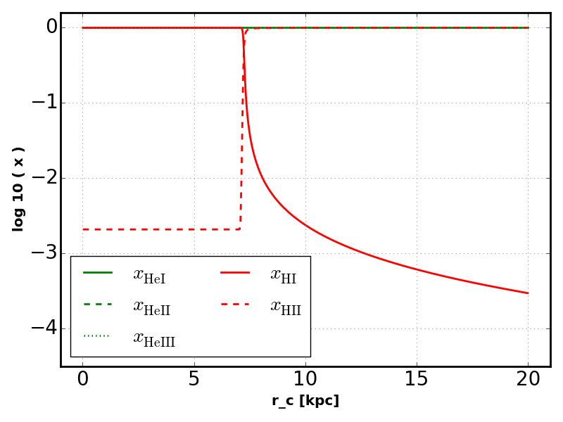
Background Sphere - RT - Case A - Mono - Fixed T
Polychromatic
Adding higher energy photons smoothes the hydrogen ionization front and produces structure in the helium ionization fractions.
key = 'rt_caseA_poly_fixT'

spheres[key] = ra.SphereBgnd(
    Edges, T, nH, nHe, src_hm12 )

plot_sphere_x( spheres[key], 'bgnd_' + key + '.png' )
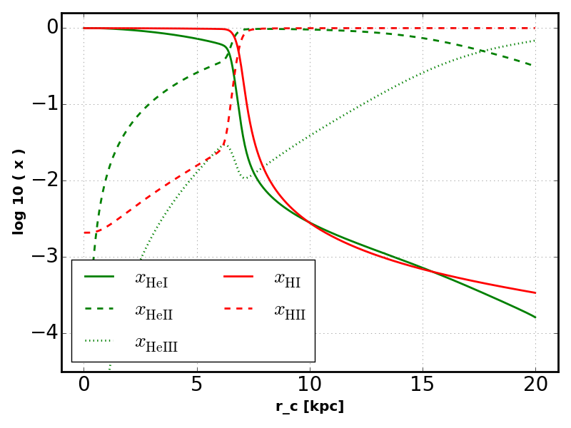
Background Sphere - RT - Case A - Poly - Fixed T
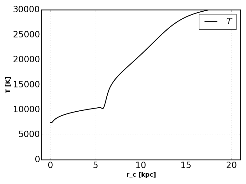
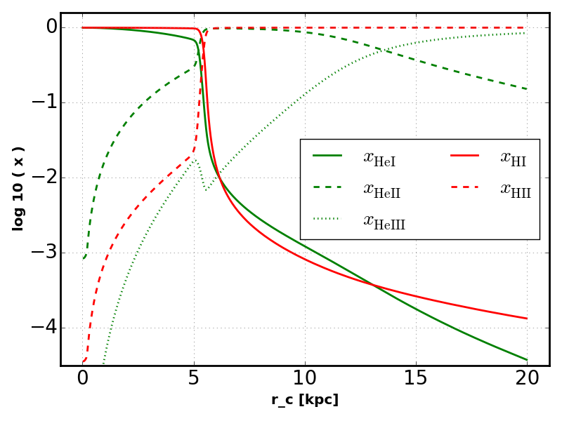
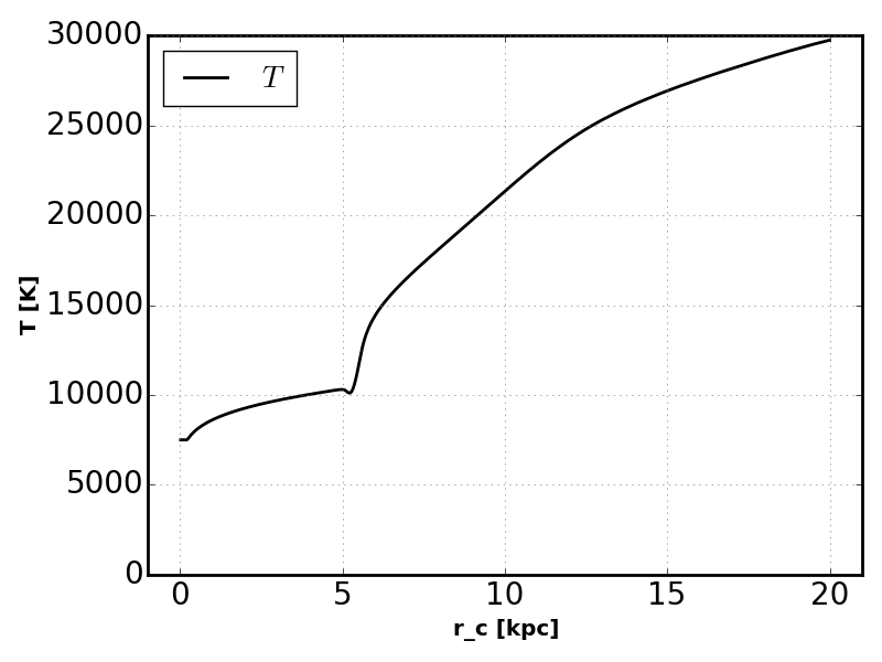
Equilibrium Temperature
If we now allow the radiation to heat the outer layers of the sphere we see some differences in the ionization profiles.
key = 'rt_caseA_poly_evoT'

spheres[key] = ra.SphereBgnd(
    Edges, T, nH, nHe, src_hm12, find_Teq=True, z=3.0 )

plot_sphere_x( spheres[key], 'bgnd_' + key + '.png' )
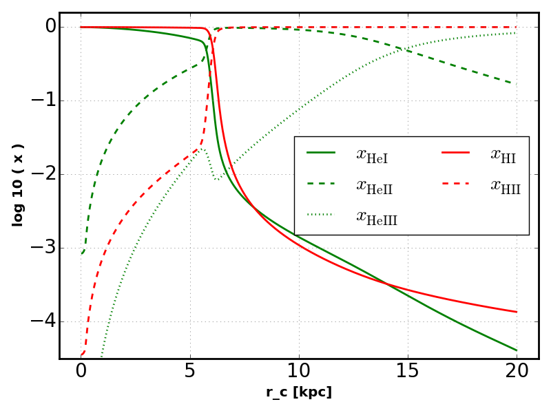
Background Sphere - RT - Case A - Poly - Equilibrium T
Background Sphere - RT - Case A - Poly - Equilibrium T
Recombination Radiation
We can also calculate the transfer of recombination radiation.
key = 'rt_isotropic_poly_evoT'

spheres[key] = ra.SphereBgnd( Edges, T, nH, nHe, src_hm12,
    find_Teq=True, z=3.0, rec_meth='isotropic' )

plot_sphere_x( spheres[key], 'bgnd_' + key + '.png' )
Background Sphere - RT - Isotropic - Poly - Equilibrium T
Background Sphere - RT - Isotropic - Poly - Equilibrium T
References
| [HM12] | http://arxiv.org/abs/1105.2039 |