Slab Examples¶

In this section we will go thourgh some concrete examples using SlabPln, Slab2Pln, and Slab2Bgnd. These classes model slab geometries with radiation incident from one or both sides respectively. First we will compare our Rabacus integrated solutions to a closed form analytic expression. Next we will examine, in steps, the more complicated scenarios that can be solved using Rabacus.

Preparation¶

Import Packages¶

The following examples require three python packages to be imported,

import numpy as np
import pylab as plt
import rabacus as ra

Plotting Functions¶

We will be making several plots during the course of these examples. In order to facilitate this, we will define a few convenience functions here,

def plot_slab_analytic( s, ana, fname ):
  """ put plot of analytic vs. rabacus solution into fname """

  plt.figure()
  s.Edges.units = 'kpc'
  s.z_c.units = 'kpc'
  xx = s.z_c
  L = s.Edges[-1]

  ana.L.units = 'kpc'

  plt.plot( xx, np.log10( s.xH1 ),
            color='red', ls='-', label = r'$x_{\rm HI}$' )
  plt.plot( xx, np.log10( s.xH2 ),
            color='red', ls='--', label = r'$x_{\rm HII}$' )

  plt.scatter( ana.L, np.log10( ana.xH1 ), s=20,
               color='black', marker='o', label='analytic' )

  plt.xlim( -L/20, L+L/20 )
  plt.xlabel( 'z_c [kpc]' )

  plt.ylim( -4.0, 0.2 )
  plt.ylabel( 'log 10 ( x )' )

  plt.grid()
  plt.legend(loc='best', ncol=2)
  plt.tight_layout()
  plt.savefig( 'doc/img/x_' + fname )


def plot_slab_x( s, fname, plot_H=True, plot_He=True ):
  """ put plot of ionization fractions from sphere `s` into fname """

  plt.figure()
  s.Edges.units = 'kpc'
  s.z_c.units = 'kpc'
  xx = s.z_c
  L = s.Edges[-1]

  if plot_He:
      plt.plot( xx, np.log10( s.xHe1 ),
                color='green', ls='-', label = r'$x_{\rm HeI}$' )
      plt.plot( xx, np.log10( s.xHe2 ),
                color='green', ls='--', label = r'$x_{\rm HeII}$' )
      plt.plot( xx, np.log10( s.xHe3 ),
                color='green', ls=':', label = r'$x_{\rm HeIII}$' )

  if plot_H:
      plt.plot( xx, np.log10( s.xH1 ),
                color='red', ls='-', label = r'$x_{\rm HI}$' )
      plt.plot( xx, np.log10( s.xH2 ),
                color='red', ls='--', label = r'$x_{\rm HII}$' )

  plt.xlim( -L/20, L+L/20 )
  plt.xlabel( 'z_c [kpc]' )

  plt.ylim( -4.0, 0.2 )
  plt.ylabel( 'log 10 ( x )' )

  plt.grid()
  plt.legend(loc='best', ncol=2)
  plt.tight_layout()
  plt.savefig( 'doc/img/x' + fname )


def plot_slab_T( s, fname ):
  """ put plot of temperature from sphere `s` into fname """

  plt.figure()
  s.Edges.units = 'kpc'
  s.z_c.units = 'kpc'
  xx = s.z_c
  L = s.Edges[-1]

  plt.plot( xx, s.T,
            color='black', ls='-', label = r'$T$' )

  plt.xlim( -L/20, L+L/20 )
  plt.xlabel( 'z_c [kpc]' )

  plt.ylim( 8.0e3, 2.6e4 )
  plt.ylabel( 'T [K]' )

  plt.grid()
  plt.legend(loc='best')
  plt.tight_layout()
  plt.savefig( 'doc/img/T_' + fname )

Create Sources¶

Next we will setup two plane parallel radiation sources, one with [HM12] spectrum at z = 3.0 between 1 and 400 Rydbergs, and another with a monochromatic spectrum equal to the grey HI energy of 16.9 eV. Note that we calculate the q_mono value for the monochromatic spectrum using the threshold ionization energy of hydrogen stored in the source itself. This eliminates small difference due to varying levels of precision when people discuss the hydrogen ionizing threshold.

z = 3.0

q_min = 1.0
q_max = 4.0e2
src_hm12 = ra.PlaneSource( q_min, q_max, 'hm12', z=z )

q_mono = src_hm12.grey.E.H1 / src_hm12.th.E_H1
q_min = q_mono
q_max = q_mono
src_mono = ra.PlaneSource( q_min, q_max, 'monochromatic' )
src_mono.normalize_H1i( src_hm12.thin.H1i )

Solution Container¶

We also initialize a dictionary to hold our results,

slabs = {}

Closed Form Solutions¶

Setup¶

In the appendix of [Altay13], we presented a closed form analytic solution for a semi-infinite constant density and temperature pure hydrogen slab with monochromatic plane parallel radiation incident from one side. That solution is implemented in Rabacus and can be used to verify the ray tracing solution. To begin, we define a slab,

Nl = 512
T = np.ones(Nl) * 1.0e4 * ra.u.K

Lslab = 1.5e2 * ra.u.kpc
Edges = np.linspace( 0.0 * ra.u.kpc, Lslab, Nl+1 )

Yp = 0.24
nH = np.ones(Nl) * 2.2e-3 / ra.u.cm**3
nHe = nH * 0.25 * Yp / ( 1.0 - Yp )
nHe_null = np.ones(Nl) * 1.0e-15 / ra.u.cm**3

Optically Thin¶

The simplest possible solution is the optically thin solution with a fixed case A fraction. We will briefly examine this solution before proceeding to the closed form analytic comparison.

key = 'thin_caseB_mono_fixT'

slabs[key] = ra.Slab(
    Edges, T, nH, nHe, src_mono, fixed_fcA=0.0, thin=True )

plot_slab_x( slabs[key], 'slab_' + key + '.png', 'I' )

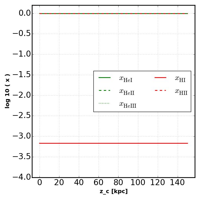
Slab - Thin - Case B - Mono - Fixed T

The solid green line and dashed red line overlap at the top of the plot. The monochromatic spectrum produces no helium ionizing photons and the temperature is not high enough to cause appreciable collisional ionization. Plane parallel radiation has no geometric dillusion factor and so we recover constant ionization fractions. The lines for singly and doubly ionized helium are off the plot towards the bottom.

Monochromatic Slab¶

Next we use Rabacus to produce a closed form solution and compare that to a solved slab with the same parameters.

ana = ra.solvers.AnalyticSlab(
  nH[0], T[0], src_hm12.thin.H1i, y=0.0, fcA=0.0 )
ana.set_E( src_hm12.grey.E.H1 )

key = 'rt_caseB_mono_fixT'
slabs[key] = ra.Slab(
    Edges, T, nH, nHe, src_mono, fixed_fcA=0.0 )

plot_slab_analytic( slabs[key], ana, 'slab_analytic.png' )

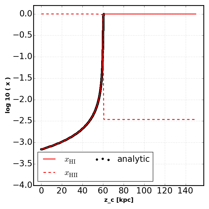
Slab - RT - Case B - Mono - Fixed T

The closed form solution is actually an inverse solution. In other words, for a given neutral fraction, it returns a depth into the slab. The points for the closed form solution are produced by creating a uniform (in log space) sampling of neutral fractions and then calculating a depth for each one. This is why the closed form solution does not continue all the way to the right of the plot.

Slab 1¶

Polychromatic Slab¶

Having verified the agreement between the closed form solution and Rabacus, we proceed to add complexity to the problem. In this section we will use the polychromatic source which will smooth the hydrogen ionization front and add structure to the helium ionization fractions,

key = 'rt_caseB_hm12_fixT'

slabs[key] = ra.Slab(
    Edges, T, nH, nHe, src_hm12, fixed_fcA=0.0 )

plot_slab_x( slabs[key], 'slab_' + key + '.png' )

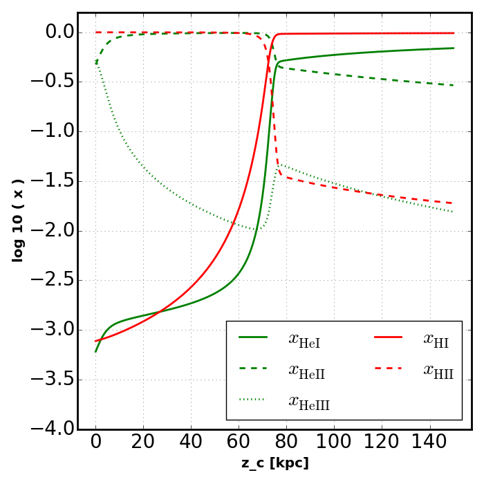
Slab - RT - Case B - HM12 - Fixed T

Equilibrium Temperature¶

In this section we will solve for the equilibrium temperature as well as the equilibrium ionization fractions.

key = 'rt_caseB_hm12_evoT'

slabs[key] = ra.Slab(
    Edges, T, nH, nHe, src_hm12, fixed_fcA=0.0, find_Teq=True, z=z )

plot_slab_x( slabs[key], 'slab_' + key + '.png', )
plot_slab_T( slabs[key], 'slab_' + key + '.png', )

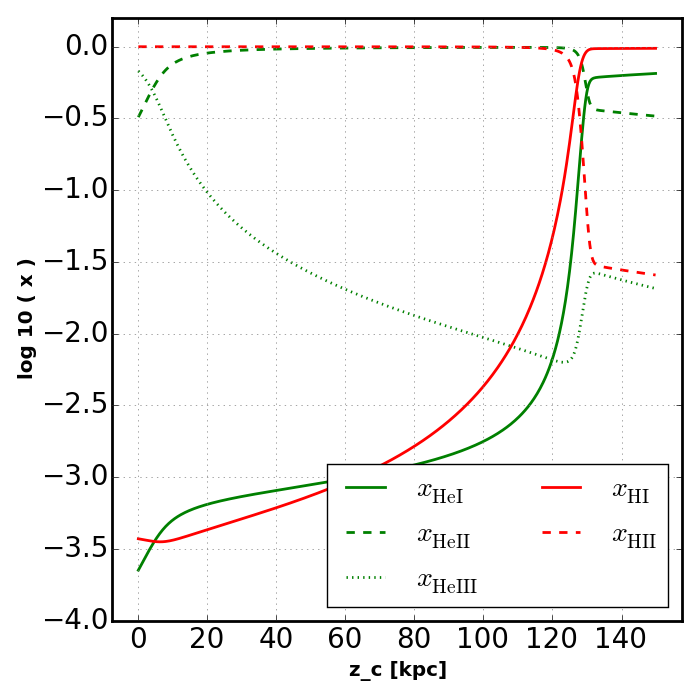
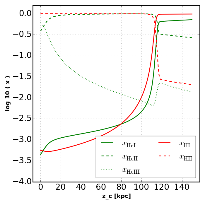
Slab - RT - Case B - HM12 - Equilibrium T

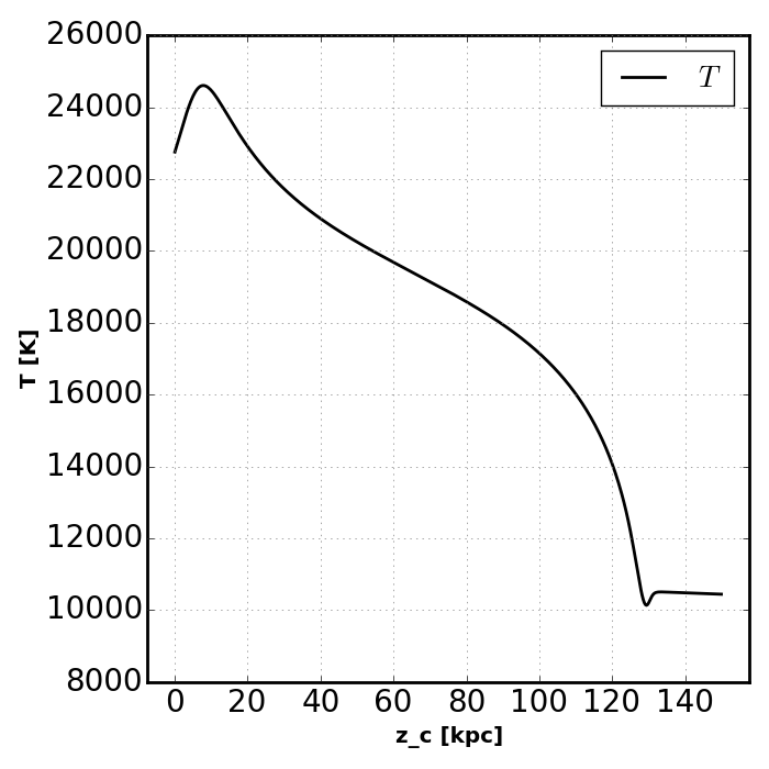
Slab - RT - Case B - HM12 - Equilibrium T

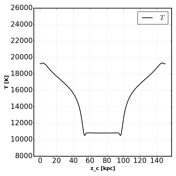
Note how the increased temperatures near the illuminated side of the slab push the ionization fronts deeper into the slab. Also notice how the temperature does not peak at the surface of the slab. This is because HeII is more effective at photoheating than other ions. However, slightly deeper into the slab the global attenuation of the radiation leads to a decline in temperature.

Recombination Radiation¶

Finally we include transfer of recombination radiation.

key = 'rt_ray_hm12_evoT'

slabs[key] = ra.Slab(
    Edges, T, nH, nHe, src_hm12, rec_meth='ray', find_Teq=True, z=z )

plot_slab_x( slabs[key], 'slab_' + key + '.png', )
plot_slab_T( slabs[key], 'slab_' + key + '.png', )

Slab - RT - Thresh - HM12 - Equilibrium T

Slab - RT - Thresh - HM12 - Equilibrium T

Slab 2¶

We can repeat all of the above problems with radiation incident from both sides instead of just one. In these cases, the flux from the plane source is split and half is incident from each side.

Monochromatic Slab¶

key = '2_rt_caseB_mono_fixT'

slabs[key] = ra.Slab2(
    Edges, T, nH, nHe, src_mono, fixed_fcA=0.0 )

plot_slab_x( slabs[key], 'slab_' + key + '.png', )

Slab2 - RT - Case B - Mono - Fixed T

Polychromatic Slab¶

key = '2_rt_caseB_hm12_fixT'

slabs[key] = ra.Slab2(
    Edges, T, nH, nHe, src_hm12, fixed_fcA=0.0 )

plot_slab_x( slabs[key], 'slab_' + key + '.png' )

Slab2 - RT - Case B - HM12 - Fixed T

Equilibrium Temperature¶

key = '2_rt_caseB_hm12_evoT'

slabs[key] = ra.Slab2(
    Edges, T, nH, nHe, src_hm12, fixed_fcA=0.0, find_Teq=True, z=z )

plot_slab_x( slabs[key], 'slab_' + key + '.png', )
plot_slab_T( slabs[key], 'slab_' + key + '.png', )

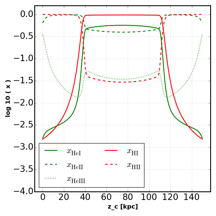
Slab2 - RT - Case B - HM12 - Equilibrium T

Slab2 - RT - Case B - HM12 - Equilibrium T

Recombination Radiation¶

key = '2_rt_ray_hm12_evoT'

slabs[key] = ra.Slab2(
    Edges, T, nH, nHe, src_hm12, rec_meth='ray', find_Teq=True, z=z )

plot_slab_x( slabs[key], 'slab_' + key + '.png', )
plot_slab_T( slabs[key], 'slab_' + key + '.png', )

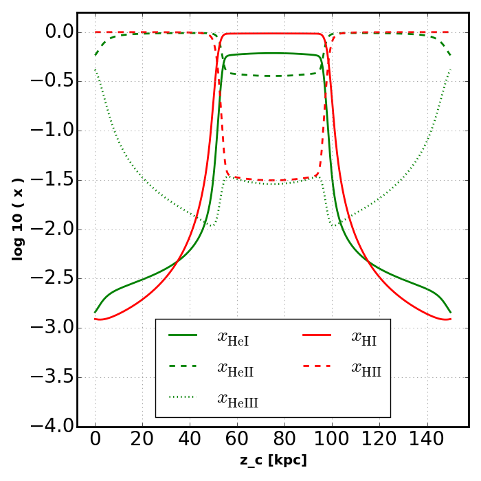
Slab2 - RT - Thresh - HM12 - Equilibrium T

Slab2 - RT - Thresh - HM12 - Equilibrium T

References¶

[Altay13]

http://arxiv.org/abs/1304.4235

[HM12]

http://arxiv.org/abs/1105.2039