rabacus.cosmology.mass_function package
Submodules
rabacus.cosmology.mass_function.mass_function module
A halo mass function module. See the following reference for a discussion, http://adsabs.harvard.edu/abs/2007ApJ...671.1160L
-
class
rabacus.cosmology.mass_function.mass_function.MassFunction(cosmo, tf)[source]¶ A mass function class. During initialization the normalization of the power spectrum is set to match the sigma8 from cosmo.
Args:
cosmo (
Cosmology): an instance of the cosmology class.tf (class): an instance of a transfer function class. For example,
TransferBBKS.cosmo is an instance of Cosmology and tf is an instance of TransferFunction
-
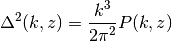
Delta2k(k, z)[source]¶ Dimensionless power spectrum,
Args:
k (real or array): wavenumber.
z (real): redshift
-
W2kR(k, R)[source]¶ The square of the fourier transform of a real space spherical top hat filter.
Args:
k (real or array): wavenumber.
R (real): filter scale.
![W^2 = \left[ \frac{ 3 j_1(x) }{ x } \right]^2, \, x = k R \\
j_1 = [\sin(x) - x \cos(x)] \, x^{-2}](_images/math/718be52b209c7553729664ef28a1557013ca476f.png)
-
W2lnkR(lnk, R)[source]¶ The square of the fourier transform of a real space spherical top hat filter as a function of the natural log of k.
Args:
lnk (real or array): natural log of wavenumber, ln( k [h/Mpc] ).
R (real): filter scale.
-
WkR(k, R)[source]¶ The fourier transform of a real space spherical top hat filter.
Args:
k (real or array): wavenumber.
R (real): filter scale.
![W = \frac{ 3 j_1(x) }{ x }, \, x = k R \\
j_1 = [\sin(x) - x \cos(x)] \, x^{-2}](_images/math/bebf1e46db5922d45c5ae8e09da9a41e62f217bc.png)
-
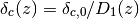
calc_mf(z, fit='Warren06')[source]¶ Calculate mass function from high to low mass. The only redshift dependence is in f(sigma) via a rescaling of sigma
-
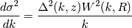
dsig2_dk(k, R, z)[source]¶ Integrand for calculation of sigma^2. Inputs k and R must have units.
Args:
k (real or array): wavenumber.
R (real): filter scale.
z (real): redshift
-
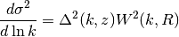
dsig2_dlnk(lnk, R, z)[source]¶ Input is ln(k) which is unitless but k must have units of h/Mpc
Args:
lnk (real or array): wavenumber, ln( k [h/Mpc] ).
R (real): filter scale.
z (real): redshift
-
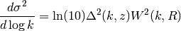
dsig2_dlogk(logk, R, z)[source]¶ Input is log10(k) which is unitless but k must have units of h/Mpc
Args:
logk (real or array): wavenumber, log10( k [h/Mpc] )
R (real): filter scale.
z (real): redshift
-
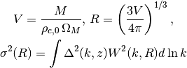
map_sig2_R(nbins=200)[source]¶ Map out the relationship between sigma^2 and R. In this routine we map out the relationship at z=0 and assume that different redshifts can be accomodated through a simple scaling with the growth function D1(z).
-
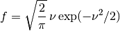
mult_func(sigma_in, z, fit='Warren06')[source]¶ The multiplicity function
 . This function
determines the shape of the mass function given the variation of
. This function
determines the shape of the mass function given the variation of
 with scale. The variable fit determines the form
of the multiplicity function. A convenient variable is
with scale. The variable fit determines the form
of the multiplicity function. A convenient variable is
 . The following values for fit
lead to the following multiplicity funcitons,
. The following values for fit
lead to the following multiplicity funcitons,-
-
![f = A \sqrt{ \frac{2a}{\pi} } [1 + (a \nu^2)^{-p}]
\nu \exp(-a \nu^2/2)
A = 0.3222, \, a = 0.75, \, p = 0.3](_images/math/1226a258ca48db18566513bbab8fa042b6f7fb47.png)
Jenkins01: Jenkins 01
Warren06: Warren 06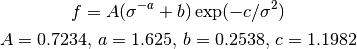
Tinker08: Tinker 08![f = A \left[ \left( \frac{\sigma}{b} \right)^{-a}
+ 1 \right] \exp(-c/\sigma^2)
\Delta=300
A = 0.1 \, \log \Delta - 0.05
a = 1.43 + ( \log \Delta - 2.3 )^{1.5}
b = 1.00 + ( \log \Delta - 1.6 )^{-1.5}
c = 1.20 + ( \log \Delta - 2.35 )^{1.6}](_images/math/93bb4b0be78693a40903424a5ac92d7685068c47.png)
-
-
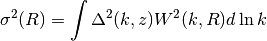
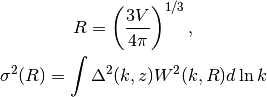
sigma2_M(M, z)[source]¶ Variance of density field smoothed on scale V
Args:
V (real): filter scale.
z (real): redshift
-
Module contents
Mass function package.