Pendulum
One-line summary: Module for studying the period of a pendulum.
Abstract: Based on a single photo-gate, it allows the measurement of the period of a pendulum and the transit time at the bottom of the oscillation.
Author: Luca Baldini
Executable: plasduino_pendulum.py
Dependencies: python, PyQt4, pyserial, avrdude, arduino.
Shield: lab1
Sketch: sktchDigitalTimer
Introduction
The aim of this simple experiment is studying the period of a pendulum
dropping the small-angle approximation and investigating its dependency on
the amplitude of the oscillation.
The pendulum and its equations are studied in details in general physics
course and this experiment is designed for students that are somewhat
familiar with them. A deep knowledge of all general-case mathematics is not
required, the simple pendulum in one dimension is enough and can be learned
in textbook or even following this
link
(and references therein).
In the following we will show an example of the kind of measurements that we
can do in this experiment. This is mainly for illustrative and didactic
purpose. A deep investigation of plasduino performance will not be done, but
we can have an idea on the quality of this setup from the discussion on the
uncertainties in the the results.
The pendulum and the acquisition system
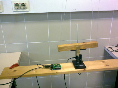
The experimental apparatus (shown in the picture on the right) is a pendulum
that consist of a mass suspended with 4 wires in a way that it can swing
always in the same plane. An optical gate is placed below the pendulum as
close as possible to the pendulum's equilibrium position.
A small flag (made of a piece of paper) is attached to the pendulum's mass
and close the optical link of the gate while the pendulum pass through.
The optical link is connected to Arduino
via the D0 input of the lab1 shield.
Arduino is configured to trigger on each transition of the optical gate
output signal and sends the timing information of each transition to the PC.
Arduino timer used in this experiment has a resolution of 4 us (relative to
Adruino internal clock), but given other effects, like jitters on the optical
gate signal, we can assume a timing resolution of the order of 10 us.
The acquisition software stores the information on the transit time and
evaluate the pendulum period (from 2 subsequent passes) and the transit time
of the pendulum flag.
Period as a function of the amplitude
For small angle of oscillations the period T of the pendulum depends solely on the length of the pendulum. For larger oscillation amplitudes θ the period becomes larger and can be described in expansion series of the maximum angle of oscillation.
We can let the pendulum oscillate from a large angle, the friction with the air will dissipate energy and will reduce the maximum oscillation amplitude as a function of time. For small time span (few seconds or, one or two complete oscillations), we can neglect the effect of the friction and assume the formula T(θ) for the ideal case. Moreover we can estimate the amplitude θ from the conservation of energy by knowing the speed of the pendulum when it crosses its equilibrium point. This speed is obtained dividing the width of the flag by its transit time.
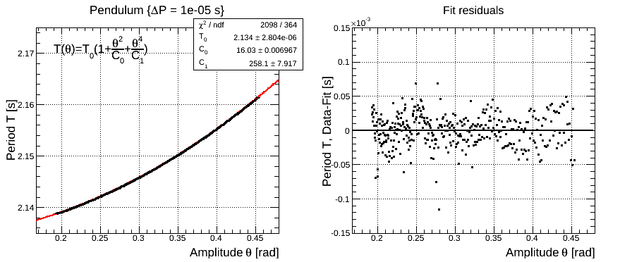
In the figure above we plot the experimental values of T as a function of θ and we compare the theoretical expectations via a fit. We assume an uncertainly on the period of 10 us and neglect the uncertainty on the oscillation amplitude. We fitted the T(θ) expansion up to the second order and keep the period for small-angle oscillation and the two coefficients for θ2 and θ4 free.x
The coefficient of the first term is in agreement with the expected value of 16 to better than 1%, although the uncertainty on the fitted value seems to be underestimate. This may be a consequence of neglecting the uncertainly on θ in the fit. Similar considerations hold for the coefficient of the second term, whose value is in agreement with the expected value of 3072/11 to better than 10%.
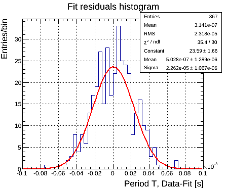
The plot of the residuals from the fitted function shows a reasonably flat trend around zero. The histogram of the residuals (shown on the right) can be described with a gaussian function, confirming a good quality of the fit. Notice that the χ2 of the fit is not a reliable indicator since we are not using good estimate of the uncertainty of the data point. As an example, using at theoretical model with only one term expansion would show a clear trend in the residual plot indicating that the model is not accurate enough.
Discussion of the uncertainties
In this work we considered only the uncertainties on the period and used 10 us as a reasonable estimate, without a comprehensive calibration of the apparatus. The rms of the residuals histograms confirms that this value is a good estimate of the order of magnitude of the period uncertainly. For a better measurements we should consider not only the intrinsic resolution of Arduino's timer but also the jitters of the optical gate signal and the accuracy of Arduino's clock (and it's drift with ambient temperature).
One possible systematic effect that is worth mentioning is that the position of the optical gate must be as close as possible to the pendulum equilibrium position. A small shift or rotation would make the estimation of θ more complicated with the final effect of an artificial increase the residual distribution rms. The data used here are taken with the same setup used by students and the perfect alignment of the optical gate was not checked.
There are several and more advanced studies that can be done with this apparatus. As an example the period or amplitude of oscillations can be studied as a function of time and modeled using different form of damping force. A second option is to estimate and include the uncertainty on the amplitude. In this work we wanted to avoid the complication of uncertainties on both axis in the fitting algorithms. The main consequence is that the uncertainty on the fitted parameters is underestimate. It is not hard to show that propagating the uncertainties on the pendulum length (~1 cm) and on the flag width (0.005 cm with a Vernier caliper) and using a fit with e.g. the effective variance method, the resulting coefficients agree with the theoretical ones to less than 1 σ.