Dice
One-line summary: Standalone module for throwing dice.
Abstract: Based on the python pseudo-random number generator, the program allows to simulate an arbitrary number of throws of an arbitrary number of dice, the sum of the dice being the variable of interest.
Author: Luca Baldini
Executable: plasduino_dice.py
Introduction
This module is designed to explain and verify the Central limit theorem stating that (under quite weak assumption) the distribution of the sum of random variables tends to a Gaussian as the number of variables increase. This module simply simulate the extraction of k dice N times and produce the distribution of the output. In the following we show an example of what can be done.
Mote-Carlo experiments

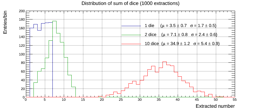
The easiest exercise is to simulate a different number of dice and look at the distribution of the sum. In the figure above we show the example of what happen with 1000 extractions of 1, 2 and 10 dice. Simulating 1 die is actually an excuse for a discrete uniform distribution with known n=6. All the moments are know and we expect μ=3.5 and σ2=(n2-1)/12 therefore σ~1.71 (not to be confused with the continuous uniform distribution where σ2=(b-a)2/12). The students can play with the statistics, by changing N, and evaluate the uncertainly on the experimental mean and rms change as function of N. If we sum 2 dice, we obtain a triangular distribution. This can be easily checked by evaluating all the possibility by hand. In this case both the average and the variance are twice the 1-die case. Summing 10 dice we are getting close to the Gaussian of the central limit theorem. The shape is much smoother than for the previous cases, average and variance scale as expected. A statistical test (e.g. a χ2 test) on this histogram can quantify how much a Gaussian hypothesis is appropriate. The students can change the number of dice k and evaluate the outcome of a statistical test as a function of k.

We can ask ourselves what is the distribution of the average of each extraction.
The central limit theorem predicts a Gaussian function, but we want to verify
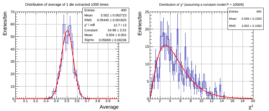
this statement directly. We simulated 1 dice N=1000 times and evaluated the average value.
We repeated this experiment 400 times to have enough statistics to sample
the distribution of the average. The histogram of these values in shown
in the left plot of the above figure. We expect a Gaussian distribution
with μ=3.5 and σ=√((n2-1)/12)/√N~0.0540 and the
result match this expectations within uncertainties.
Another interesting exercise is, for each simulation of 1 die N times,
to evaluate the χ2 with the theoretical model (in this case a simple
constant with N/6). Sampling this value several times allows to ``see'' the
χ2 distribution (in this case with d=n-1=5 degrees of freedom).
The right plot of the above figure shows the histograms of the result with the
formula of the χ2d=5 distribution.
The mean and the rms are close (within uncertainties) to the expected
μ=d and σ=√2d.