Contents
1. Data Structures
1.1. CNOgraph module
- class CNOGraph(model=None, data=None, verbose=False, **kargs)[source]
Data structure (Digraph) used to manipulate networks
The networks can represent for instance a protein interaction network.
CNOGraph is a graph data structure dedicated to the analysis of phosphorylation data within protein-protein interaction networks but can be used in a more general context. Indeed no data is required. Note that CNOGraph inherits from the directed graph data structure of networkx.
- However, we impose links between nodes to be restricted to two types:
- “+” for activation
- “-” for inhibition.
An instance can be created from an empty graph:
c = CNOGraph()
and edge can be added as follows:
c.add_edge("A", "B", link="+")
c.add_edge("A", "C", link="-")
The methods add_node() and add_edge() methods can be used to populate the graph. However, it is also possible to read a network stored in a file in cellnopt.core.sif.SIF format:
>>> from cellnopt.core import *
>>> pknmodel = cnodata("PKN-ToyPB.sif")
>>> c = CNOGraph(pknmodel)
The SIF model can be a filename, or an instance of SIF. Note for CellNOpt users that if and nodes are contained in the original SIF files, they are kept (see the SIF documentation for details).
You can add or remove nodes/edges in the CNOGraph afterwards.
As mentionned above, you can also populate data within the CNOGraph data structure. The input data is an instance of XMIDAS or a MIDAS filename. MIDAS file contains measurements made on proteins in various experimental conditions (stimuli and inhibitors). The names of the simuli, inhibitors and signals are used to color the nodes in the plotting function. However, the data itself is not used.
If you don’t use any MIDAS file as input, you can set the stimuli/inhibitors/signals manually by filling the hidden attributes _stimuli, _signals and _inhibitors.
Node and Edge attributes
The node and edge attributes can be accessed as follows (and changed):
>>> c.node['egf']
{'color': u'black',
 u'fillcolor': u'white',
 'penwidth': 2,
 u'shape': u'rectangle',
 u'style': u'filled,bold'}

>>> c.edge['egf']['egfr']
{u'arrowhead': u'normal',
 u'color': u'black',
 u'compressed': [],
 'link': u'+',
 u'penwidth': 1}
OPERATORS
CNOGraph is a data structure with useful operators (e.g. union). Note, however, that these operators are applied on the topology only (MIDAS information is ignored). For instance, you can add graphs with the + operator or check that there are identical
c = a+b
a += b
a == b
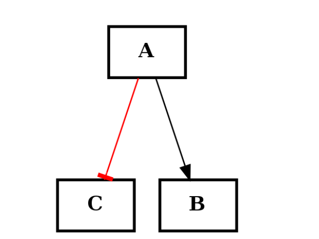
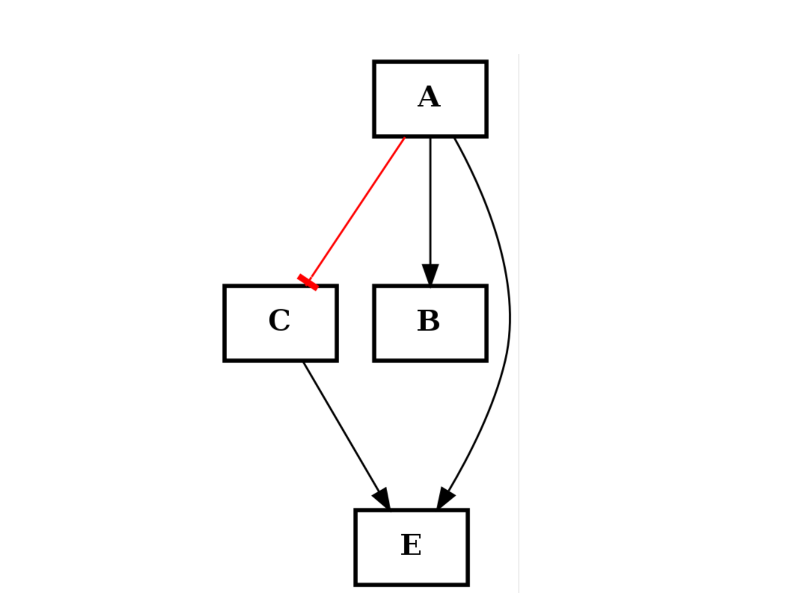
Let us illustrate the + operation with another example. Let us consider the following graphs:
from cellnopt.core import *
c1 = CNOGraph()
c1.add_edge("A","B", link="+")
c1.add_edge("A","C", link="-")
c1.plotdot()
(Source code, png, hires.png, pdf)
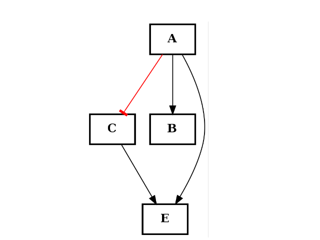
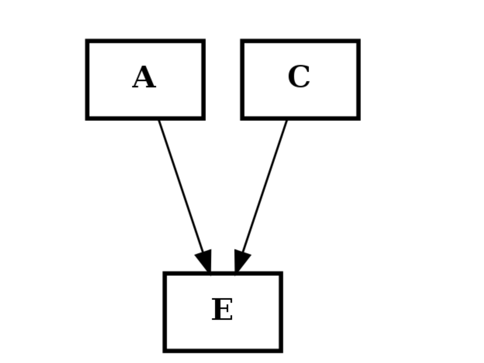
from cellnopt.core import *
c2 = CNOGraph()
c2.add_edge("A","E", link="+")
c2.add_edge("C","E", link="+")
c2.plotdot()
(Source code, png, hires.png, pdf)

(c1+c2).plotdot()
(Source code, png, hires.png, pdf)
You can also substract a graph from another one:
c3 = c1 - c2
c3.nodes()
The new graph should contains only one node (B). Additional functionalities such as intersect(), union() and difference() can be used to see the difference between two graphs.
PLOTTING
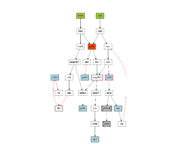
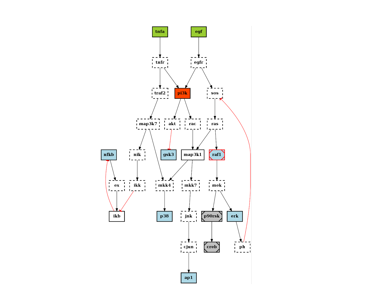
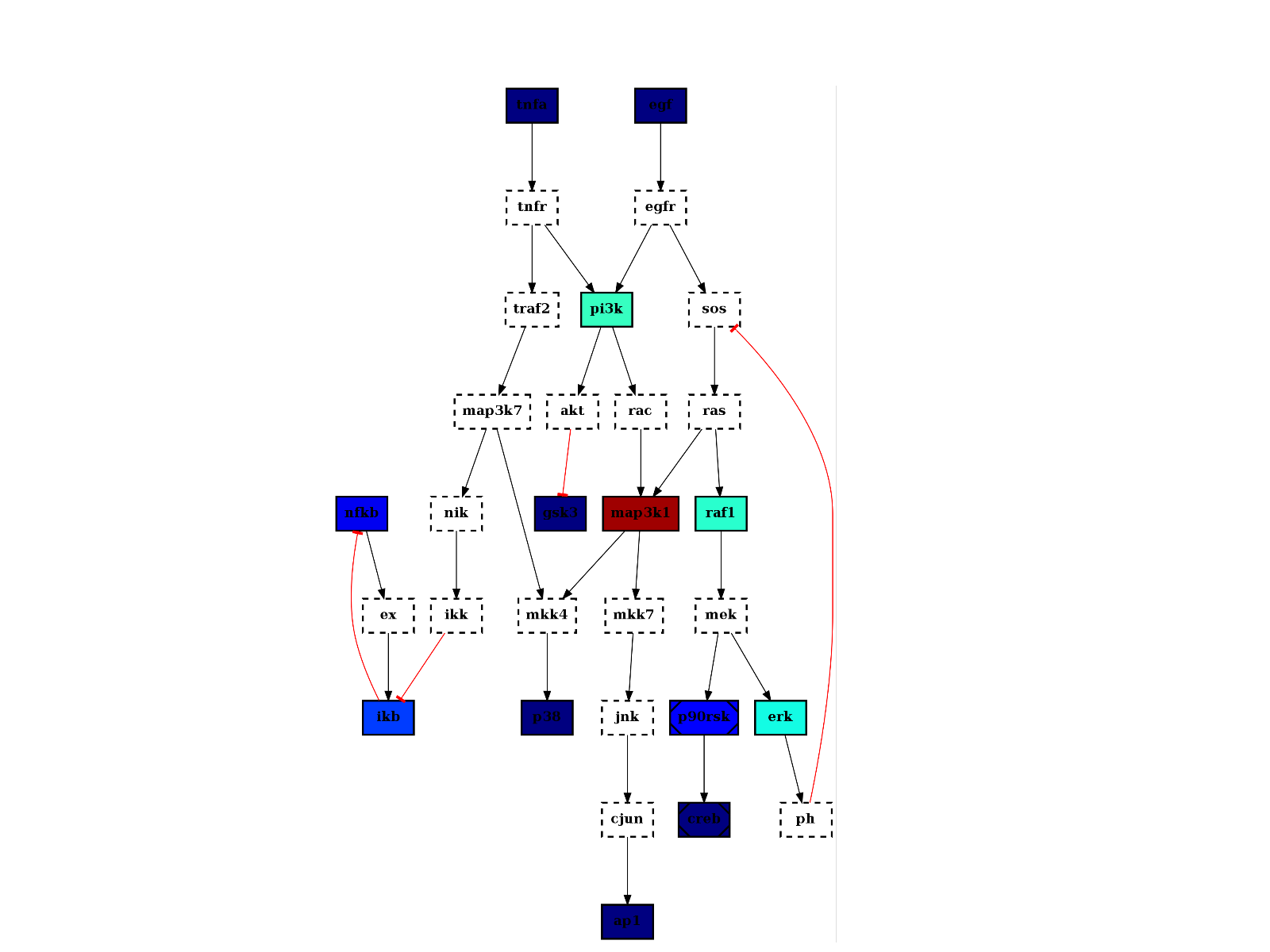
There are plotting functionalities to look at the graph, which are based on graphviz library. For instance, the plotdot() is quite flexible but has a default behaviour following CellNOptR convention, where stimuli are colored in green, inhibitors in red and measurements in blue:
from cellnopt.core import *
pknmodel = cnodata("PKN-ToyPB.sif")
data = cnodata("MD-ToyPB.csv")
c = CNOGraph(pknmodel, data)
c.plotdot()
(Source code, png, hires.png, pdf)

If you did not use any MIDAS file as input parameter, you can still populate the hidden fields _stimuli, _inhibitors, _signals.
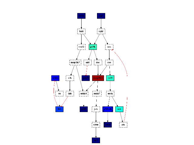
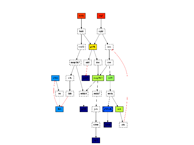
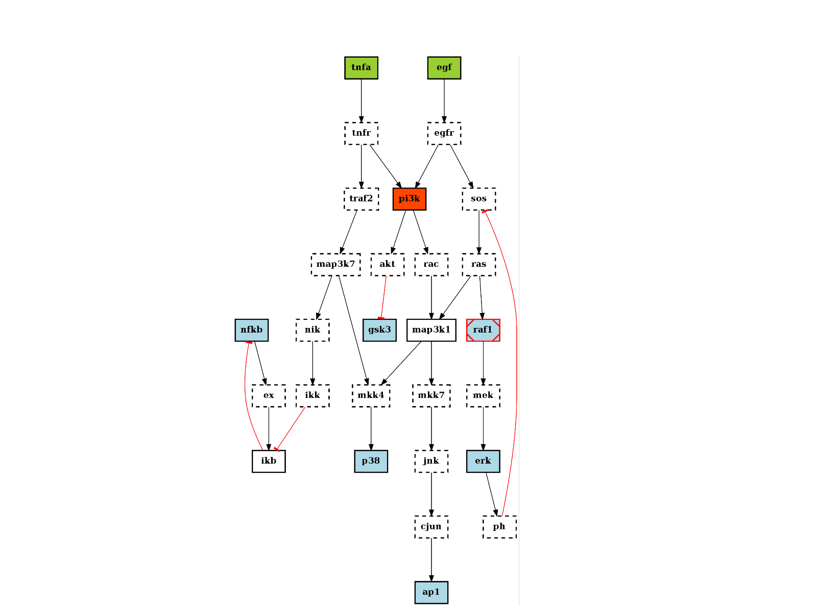
You can also overwrite this behaviour by using the node_attribute parameter when calling plotdot(). For instance, if you call centrality_degree(), which computes and populate the node attribute degree. You can then call plotdot as follows to replace the default color:
from cellnopt.core import *
pknmodel = cnodata("PKN-ToyPB.sif")
data = cnodata("MD-ToyPB.csv")
c = CNOGraph(pknmodel, data)
c.centrality_degree()
c.plotdot(node_attribute="degree")
(Source code, png, hires.png, pdf)

Similarly, you can tune the color of the edge attribute. See the plotdot() for more details.
See also
tutorial, user guide
Todo
graph attribute seems to be reset somewhere
Todo
penwidth should be a class attribute, overwritten if provided.
Todo
call findnonc only once or when nodes are changed.
Todo
reacID when a model is expanded, returns only original reactions
Constructor
Parameters: Todo
check that the celltype option works
- add_cycle(nodes, **attr)[source]
Add a cycle
Parameters: - nodes (list) – a list of nodes. A cycle will be constructed from the nodes (in order) and added to the graph.
- attr (dict) – must provide the “link” keyword. Valid values are “+”, “-” the links of every edge in the cycle will be identical.
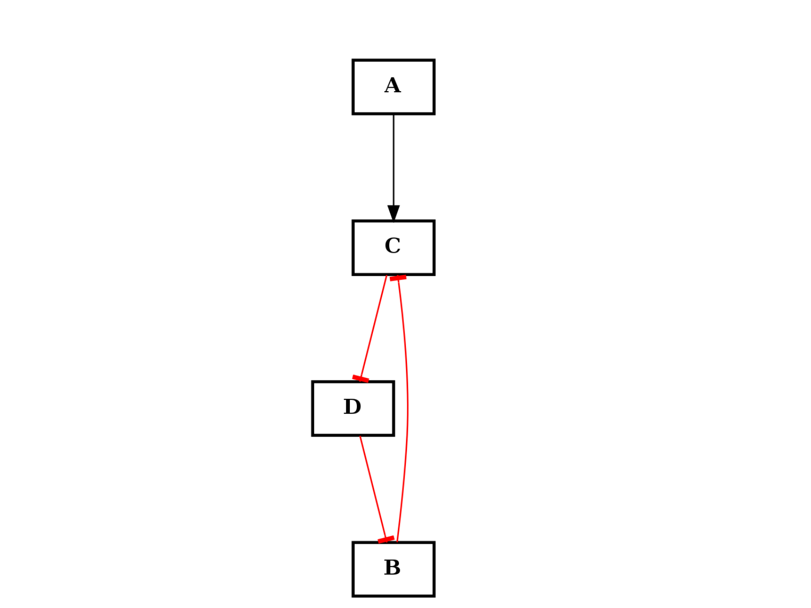
from cellnopt.core import *
c = CNOGraph()
c.add_edge("A", "C", link="+")
c.add_edge("B", "C", link="+")
c.add_cycle(["B", "C", "D"], link="-")
c.plotdot()
(Source code, png, hires.png, pdf)

Warning
added cycle overwrite previous edges
- add_edge(u, v, attr_dict=None, **attr)[source]
adds an edge between node u and v.
Parameters: - u (str) – source node
- v (str) – target node
- link (str) – compulsary keyword. must be “+” or “-“
- attr_dict (dict) – dictionary, optional (default= no attributes) Dictionary of edge attributes. Key/value pairs will update existing data associated with the edge.
- attr – keyword arguments, optional edge data (or labels or objects) can be assigned using keyword arguments. keywords provided will overwrite keys provided in the attr_dict parameter
Warning
color, penwidth, arrowhead keywords are populated according to the value of the link.
- If link=”+”, then edge is black and arrowhead is normal.
- If link=”-”, then edge is red and arrowhead is a tee
from cellnopt.core import *
c = CNOGraph()
c.add_edge("A","B",link="+")
c.add_edge("A","C",link="-")
c.add_edge("C","D",link="+", mycolor="blue")
c.add_edge("C","E",link="+", data=[1,2,3])
You can also add several edges at the same time for a single output but multiple entries:
c.add_edge("A+B+C", "D", link="+")
equivalent to
c.add_edge("A", "D", link="+")
c.add_edge("B", "D", link="+")
c.add_edge("C", "D", link="+")
Attributes on the edges can be provided using the parameters attr_dict (a dictionary) and/or **attr, which is a list of key/value pairs. The latter will overwrite the key/value pairs contained in the dictionary. Consider this example:
c = CNOGraph()
c.add_edge("a", "c", attr_dict={"k":1, "data":[0,1,2]}, link="+", k=3)
c.edges(data=True)
[('a',
'c',
    {'arrowhead': 'normal',
    'color': 'black',
    'compressed': [],
    'data': [0, 1, 2],
    'k':3
    'link': '+',
    'penwidth': 1})]
The field “k” in the dictionary (attr_dict) is set to 1. However, it is also provided as an argument but with the value 3. The latter is the one used to populate the edge attributes, which can be checked by printing the data of the edge (c.edges(data=True())
See also
special attributes are automatically set by set_default_edge_attributes(). the color of the edge is black if link is set to “+” and red otherwie.
- add_edges_from(ebunch, attr_dict=None, **attr)[source]
add list of edges with same parameters
c.add_edges_from([(0,1),(1,2)], data=[1,2])
See also
add_edge() for details.
- add_node(node, attr_dict=None, **attr)[source]
Add a node
Parameters: - node (str) – a node to add
- attr_dict (dict) – dictionary, optional (default= no attributes) Dictionary of edge attributes. Key/value pairs will update existing data associated with the edge.
- attr – keyword arguments, optional edge data (or labels or objects) can be assigned using keyword arguments. keywords provided will overwrite keys provided in the attr_dict parameter
Warning
color, fillcolor, shape, style are automatically set.
c = CNOGraph()
c.add_node("A", data=[1,2,3,]
Warning
**attr replaces any key found in attr_dict. See add_edge() for details.
Todo
currently nodes that contains a ^ sign are interpreted as AND gate and will appear as small circle. One way to go around is to use the label attribute. you first add the node with a differnt name and populate the label with the correct nale (the one that contain the ^ sign); When calling the plot function, they should all appear as expected.
- add_nodes_from(nbunch, attr_dict=None, **attr)[source]
Add a bunch of nodes
Parameters: - nbunch (list) – list of nodes. Each node being a string.
- attr_dict (dict) – dictionary, optional (default= no attributes) Dictionary of edge attributes. Key/value pairs will update existing data associated with the edge.
- attr – keyword arguments, optional edge data (or labels or objects) can be assigned using keyword arguments. keywords provided will overwrite keys provided in the attr_dict parameter
Warning
color, fillcolor, shape, style are automatically set.
See also
add_node() for details.
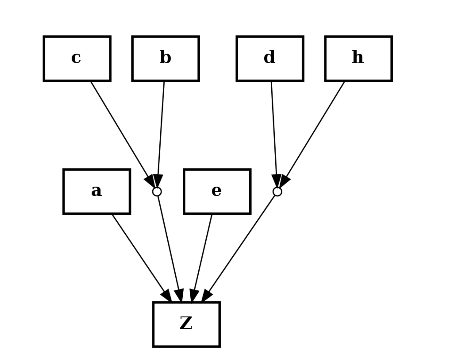
- add_reaction(reac, **edge_attributes)[source]
Add nodes and edges given a reaction
Parameters: reac (str) – a valid reaction. See below for examples Here are some valid reactions that includes NOT, AND and OR gates. + is an OR and ^ character is an AND gate:
>>> s.add_reaction("A=B")
>>> s.add_reaction("A+B=C")
>>> s.add_reaction("A^C=E")
>>> s.add_reaction("!F+G=H")
from cellnopt.core import *
c = CNOGraph()
c.add_reaction("a+b^c+e+d^h=Z")
c.plotdot()
(Source code, png, hires.png, pdf)

- adjacencyMatrix(nodelist=None, weight=None)[source]
Return adjacency matrix.
Parameters: - nodelist (list) – The rows and columns are ordered according to the nodes in nodelist. If nodelist is None, then the ordering is produced by nodes() method.
- weight (str) – (default=None) The edge data key used to provide each value in the matrix. If None, then each edge has weight 1. Otherwise, you can set it to “weight”
Returns: numpy matrix Adjacency matrix representation of CNOGraph.
Note
alias to networkx.adjacency_matrix()
See also
adjacency_iter() and adjacency_list()
- attributes = None
the attributes for nodes and edges are stored within this attribute. See CNOGraphAttributes
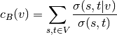
- centrality_betweeness(k=None, normalized=True, weight=None, endpoints=False, seed=None)[source]
Compute the shortest-path betweeness centrality for nodes.
Betweenness centrality of a node v is the sum of the fraction of all-pairs shortest paths that pass through v:
where
 is the set of nodes,
  is the number of
shortest
is the number of
shortest  -paths, and
  is the number of those
paths passing through some node
is the number of those
paths passing through some node  other than
  .
If
.
If  ,
,  , and if
  ,
,
 .
.Parameters: - k (int) – (default=None) If k is not None use k node samples to estimate betweeness. The value of k <= n where n is the number of nodes in the graph. Higher values give better approximation.
- normalized (bool) – If True the betweeness values are normalized by
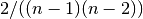 for graphs, and
 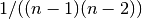 for directed graphs where
  is the number of nodes in G.
 - weight (str) – None or string, optional If None, all edge weights are considered equal.
from cellnopt.core import *
c = CNOGraph(cnodata("PKN-ToyPB.sif"), cnodata("MD-ToyPB.csv"))
c.centrality_betweeness()
c.plotdot(node_attribute="centrality_betweeness")
(Source code, png, hires.png, pdf)

See also
networkx.centrality.centrality_betweeness
- centrality_closeness(**kargs)[source]
Compute closeness centrality for nodes.
Closeness centrality at a node is 1/average distance to all other nodes.
Parameters: - v – node, optional Return only the value for node v
- distance (str) – string key, optional (default=None) Use specified edge key as edge distance. If True, use ‘weight’ as the edge key.
- normalized (bool) – optional If True (default) normalize by the graph size.
Returns: Dictionary of nodes with closeness centrality as the value.
from cellnopt.core import *
c = CNOGraph(cnodata("PKN-ToyPB.sif"), cnodata("MD-ToyPB.csv"))
c.centrality_closeness()
c.plotdot(node_attribute="centrality_closeness")
(Source code, png, hires.png, pdf)

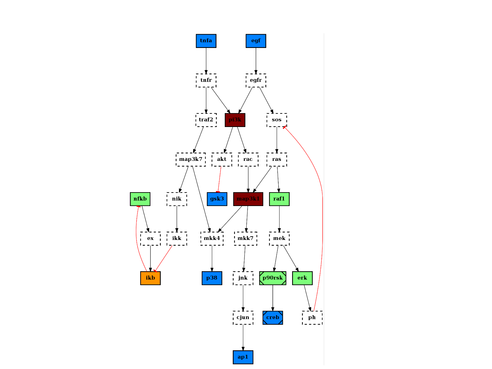
- centrality_degree()[source]
Compute the degree centrality for nodes.
The degree centrality for a node v is the fraction of nodes it is connected to.
Returns: list of nodes with their degree centrality. It is also added to the list of attributes with the name “degree_centr” from cellnopt.core import * c = CNOGraph(cnodata("PKN-ToyPB.sif"), cnodata("MD-ToyPB.csv")) c.centrality_degree() c.plotdot(node_attribute="centrality_degree")
(Source code, png, hires.png, pdf)
- clean_orphan_ands()[source]
Remove AND gates that are not AND gates anymore
When removing an edge or a node, AND gates may not be valid anymore either because the output does not exists or there is a single input.
This function is called when remove_node() or remove_edge() are called. However, if you manipulate the nodes/edges manually you may need to call this function afterwards.
- collapse_node(node)[source]
Collapses a node (removes a node but connects input nodes to output nodes)
This is different from remove_node(), which removes a node and its edges thus creating non-connected graph. collapse_node(), instead remove the node but merge the input/output edges IF possible. If there are multiple inputs AND multiple outputs the node is not removed.
Parameters: node (str) – a node to collapse. - Nodes are collapsed if there is at least one input or output.
- Node are not removed if there is several inputs and several ouputs.
- if the input edge is -, and the next is + or viceversa then the final edge if -
- if the input edge is - and output is - then final edge is +
- collapse_nodes(nodes)[source]
Collapse a list of nodes
Parameters: nodes (list) – a list of node to collapse See also
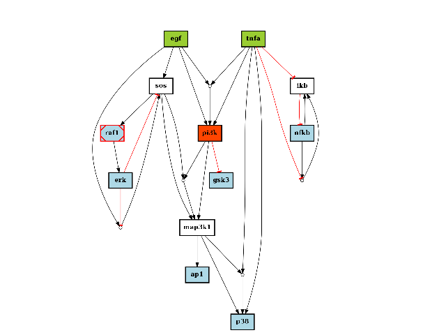
- compress()[source]
Finds compressable nodes and removes them from the graph
A compressable node is a node that is not part of the special nodes (stimuli/inhibitors/readouts mentionned in the MIDAS file). Nodes that have multiple inputs and multiple outputs are not compressable either.
from cellnopt.core import *
c = CNOGraph(cnodata("PKN-ToyPB.sif"), cnodata("MD-ToyPB.csv"))
c.cutnonc()
c.compress()
c.plotdot()
(Source code, png, hires.png, pdf)

See also
- compressable_nodes
Returns list of compressable nodes (Read-only).
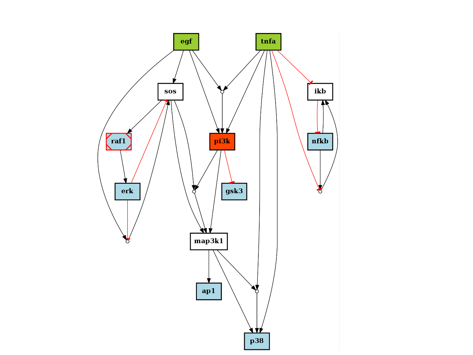
- cutnonc()[source]
Finds non-observable and non-controllable nodes and removes them.
from cellnopt.core import *
c = CNOGraph(cnodata("PKN-ToyPB.sif"), cnodata("MD-ToyPB.csv"))
c.cutnonc()
c.plotdot()
(Source code, png, hires.png, pdf)

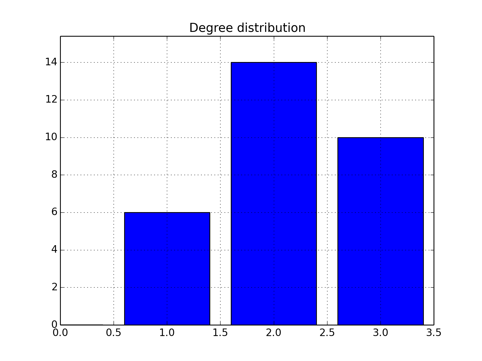
- degree_histogram(show=True, normed=False)[source]
Compute histogram of the node degree (and plots the histogram)
from cellnopt.core import *
c = CNOGraph(cnodata("PKN-ToyPB.sif"), cnodata("MD-ToyPB.csv"))
c.degree_histogram()
(Source code, png, hires.png, pdf)

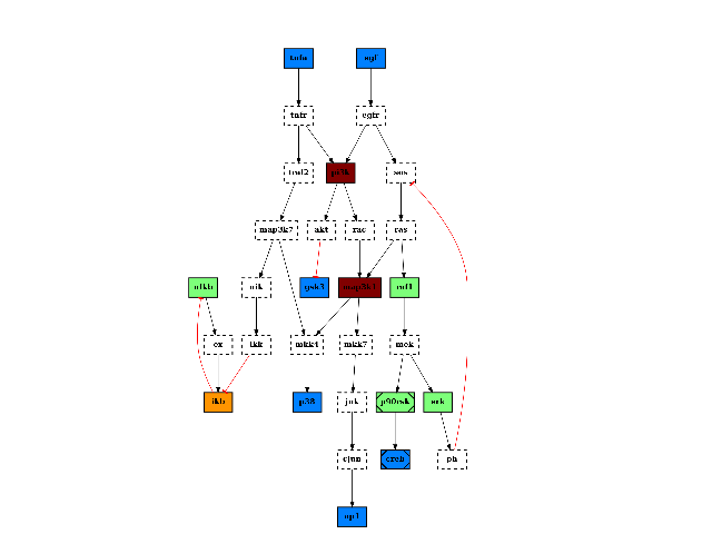
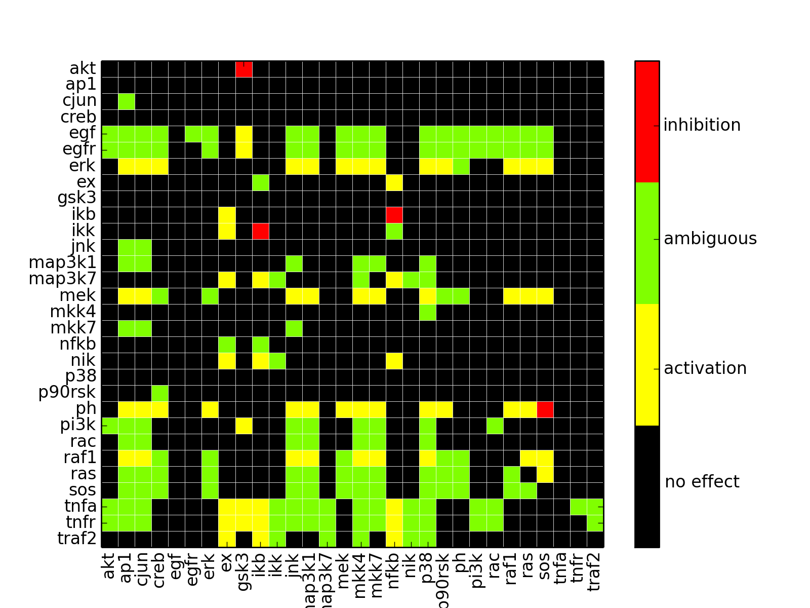
- dependencyMatrix(fontsize=12)[source]
Return dependency matrix
 = green ; species i is an activator of species j (only positive path)
- = red ; species i is an inhibitor of species j (only negative path)
- = yellow; ambivalent (positive and negative paths connecting i and j)
- = red ; species i has no influence on j
from cellnopt.core import *
c = CNOGraph(cnodata("PKN-ToyPB.sif"), cnodata("MD-ToyPB.csv"))
c.dependencyMatrix()
(Source code, png, hires.png, pdf)
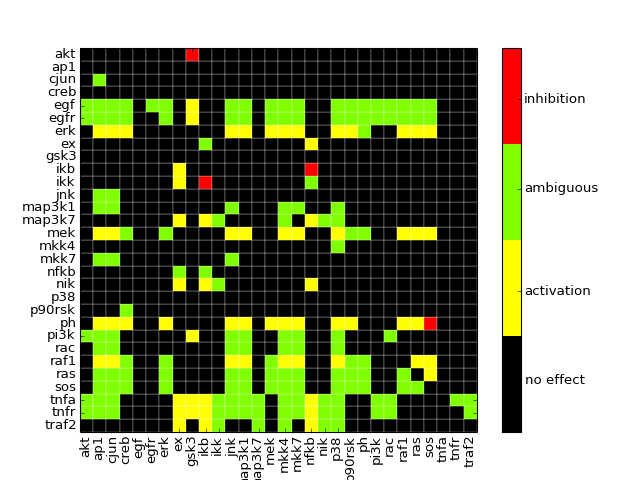
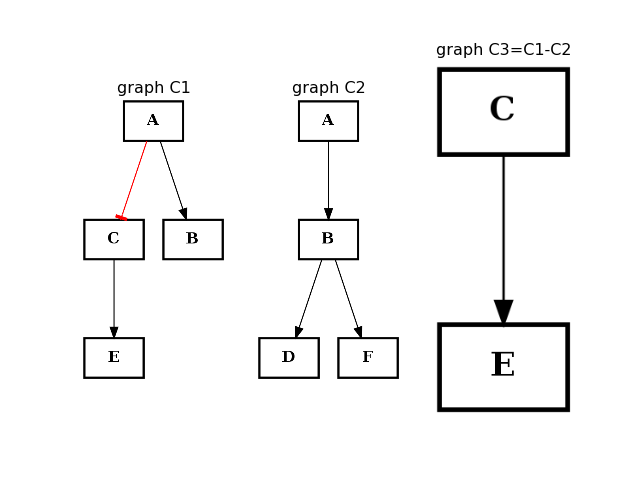
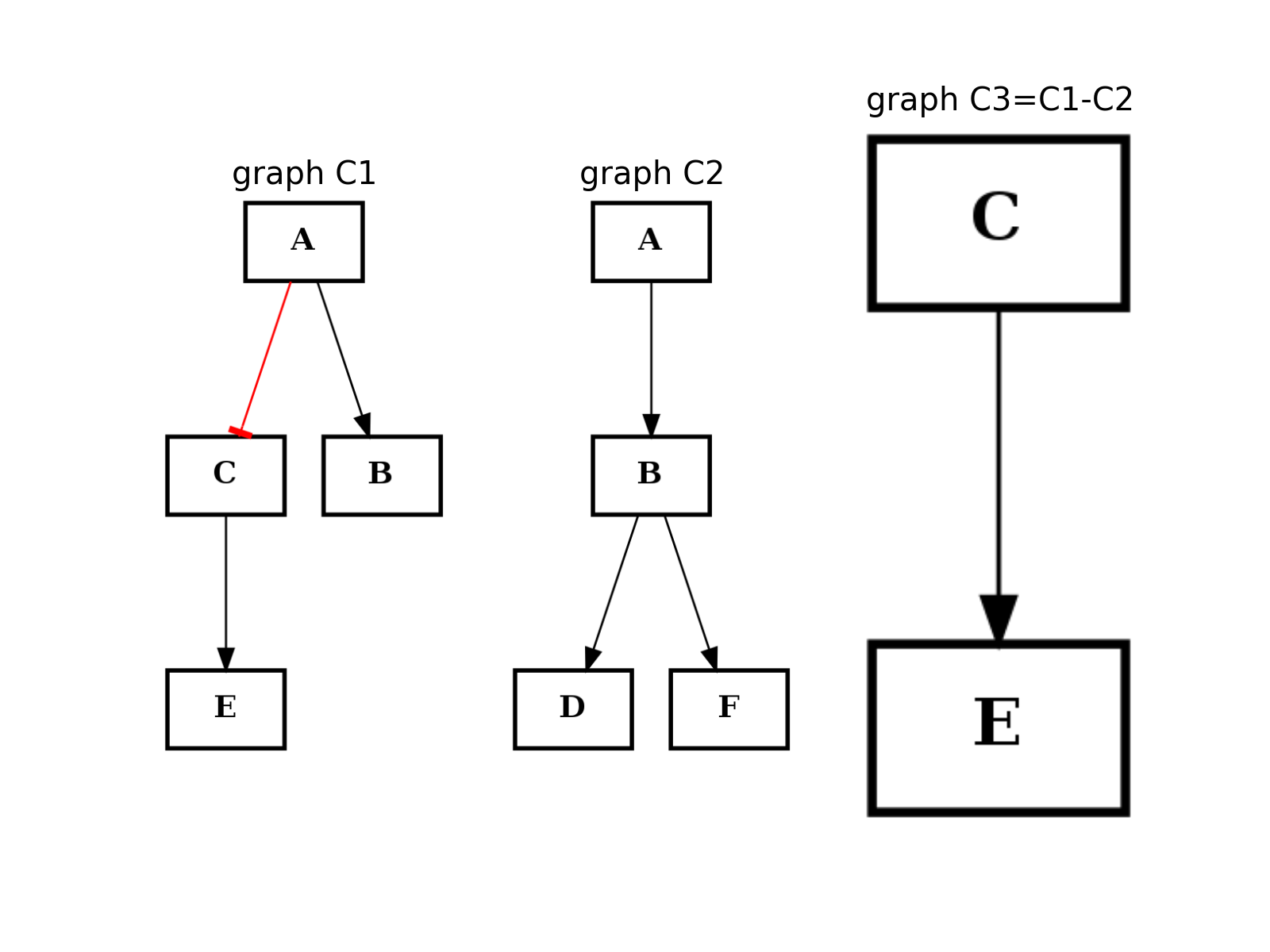
- difference(other)[source]
Return a CNOGraph instance that is the difference with the input graph
(i.e. all elements that are in this set but not the others.)
from cellnopt.core import *
from pylab import subplot, title

c1 = CNOGraph()
c1.add_edge("A", "B", link="+")
c1.add_edge("A", "C", link="-")
c1.add_edge("C", "E", link="+")
subplot(1,3,1)
title("graph C1")
c1.plotdot(hold=True)

c2 = CNOGraph()
c2.add_edge("A", "B", link="+")
c2.add_edge("B", "D", link="+")
c2.add_edge("B", "F", link="+")
subplot(1,3,2)
c2.plotdot(hold=True)
title("graph C2")

c3 = c1.difference(c2)
subplot(1,3,3)
c3.plotdot(hold=True)
title("graph C3=C1-C2")
(Source code, png, hires.png, pdf)
Note
this method should be equivalent to the - operator. So c1-c2 == c1.difference(c2)
- dot_mode
Read/Write attribute to use with plotdot2 method (experimental).
- draw(prog='dot', hold=False, attribute='fillcolor', colorbar=True, **kargs)[source]
Draw the network using matplotlib. Not exactly what we want but could be useful.
Parameters: - prog (str) – one of the graphviz program (default dot)
- hold (bool) – hold previous plot (default is False)
- attribute (str) – attribute to use to color the nodes (default is “fillcolor”).
- node_size – default 1200
- width – default 2
- colorbar (bool) – add colorbar (default is True)
Uses the fillcolor attribute of the nodes Uses the link attribute of the edges
See also
plotdot() that is dedicated to this kind of plot using graphviz
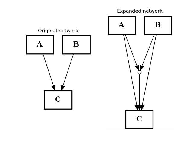
- expand_and_gates(maxInputsPerGate=2)[source]
Expands the network to incorporate AND gates
Parameters: maxInputsPerGate (int) – restrict maximum number of inputs used to create AND gates (default is 2) The CNOGraph instance can be used to model a boolean network. If a node has several inputs, then the combinaison of the inputs behaves like an OR gate that is we can take the minimum over the inputs.
In order to include AND behaviour, we introduce a special node called AND gate. This function adds AND gates whenever a node has several inputs. The AND gates can later on be used in a boolean formalism.
In order to recognise AND gates, we name them according to the following rule. If a node A has two inputs B and C, then the AND gate is named:
B^C=A
and 3 edges are added: B to the AND gates, C to the AND gates and the AND gate to A.
If an edge is a “-” link then, an ! character is introduced.
In this expansion process, AND gates themselves are ignored.
If there are more than 2 inputs, all combinaison of inputs may be considered but the default parameter maxInputsPerGate is set to 2. For instance, with 3 inputs A,B,C you may have the following combinaison: A^B, A^C, B^C. The link A^B^C will be added only if maxInputsPerGate is set to 3.
from cellnopt.core import *
from pylab import subplot, title

c = CNOGraph()
c.add_edge("A", "C", link="+")
c.add_edge("B", "C", link="+")
subplot(1,2,1)
title("Original network")
c.plotdot(hold=True)

c.expand_and_gates()
subplot(1,2,2)
c.plotdot(hold=True)
title("Expanded network")
(Source code, png, hires.png, pdf)
See also
Note
this method adds all AND gates in one go. If you want to add a specific AND gate, you have to do it manually. You can use the add_reaction() for that purpose.
Note
propagate data from edge on the AND gates.
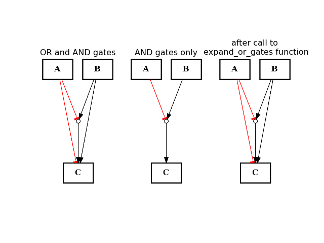
- expand_or_gates()[source]
Expand OR gates given AND gates
If a graph contains AND gates (without its OR gates), you can add back the OR gates automatically using this function.
from cellnopt.core import *
from pylab import subplot, title

c1 = CNOGraph()
c1.add_edge("A", "C", link="-")
c1.add_edge("B", "C", link="+")
c1.expand_and_gates()
subplot(1,3,1)
title("OR and AND gates")
c1.plotdot(hold=True)

c1.remove_edge("A", "C")
c1.remove_edge("B", "C")
subplot(1,3,2)
c1.plotdot(hold=True)
title("AND gates only")

c1.expand_or_gates()
subplot(1,3,3)
c1.plotdot(hold=True)
title("after call to \n expand_or_gates function")
(Source code, png, hires.png, pdf)
See also
- export2SBMLQual(filename, modelName='CellNOpt_model')[source]
Export the topology into SBMLqual and save in a file
This requires only the topology information (i.e. MIDAS content is ignored).
- export2gexf(filename)[source]
Export into GEXF format
Parameters: filename (str) – This is the networkx implementation and requires the version 1.7 This format is quite rich and can be used in external software such as Gephi.
Warning
color and labels are lost. information is stored as attributes.and should be as properties somehow. Examples: c.node[‘mkk7’][‘viz’] = {‘color’: {‘a’: 0.6, ‘r’: 239, ‘b’: 66,’g’: 173}}
- export2sif(filename)[source]
Export CNOGraph into a SIF file.
Takes into account and gates. If a species called “A^B=C” is found, it is an AND gate that is encoded in a CSV file as:
A 1 and1
B 1 and1
and1 1 C
Parameters: filename (str) – Todo
could use SIF class instead to simplify the code
- findnonc()[source]
Finds the Non-Observable and Non-Controllable nodes
- Non observable nodes are those that do not have a path to any measured species in the PKN
- Non controllable nodes are those that do not receive any information from a species that is perturbed in the data.
Such nodes can be removed without affecting the readouts.
Parameters: - G – a CNOGraph object
- stimuli – list of stimuli
- stimuli – list of signals
Returns: a list of names found in G that are NONC nodes
>>> from cellnopt.core import *
>>> from cellnopt.core.nonc import findNONC
>>> model = cnodata('PKN-ToyMMB.sif')
>>> data = cnodata('MD-ToyMMB.csv')
>>> c = CNOGraph(model, data)
>>> namesNONC = c.nonc()
Details: Using a floyd Warshall algorithm to compute path between nodes in a directed graph, this class identifies the nodes that are not connected to any signals (Non Observable) and/or any stimuli (Non Controllable) excluding the signals and stimuli, which are kept whatever is the outcome of the FW algorithm.
- get_max_rank()[source]
Get the maximum rank from the inputs using floyd warshall algorithm
If a MIDAS file is provided, the inputs correspond to the stimuli. Otherwise, (or if there is no stimuli in the MIDAS file), use the nodes that have no predecessors as inputs (ie, rank=0).
- get_node_attributes(node)[source]
Returns attributes of a node using the MIDAS attribute
Given a node, this function identifies the type of the input node and returns a dictionary with the relevant attributes found in node_attributes.attributes.
For instance, if a midas file exists and if node belongs to the stimuli, then the dicitonary returned contains the color green.
Parameters: node (str) – Returns: dictionary of attributes.
- get_same_rank()[source]
Return ranks of the nodes.
Used by plotdot/graphviz. Depends on attribute dot_mode
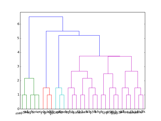
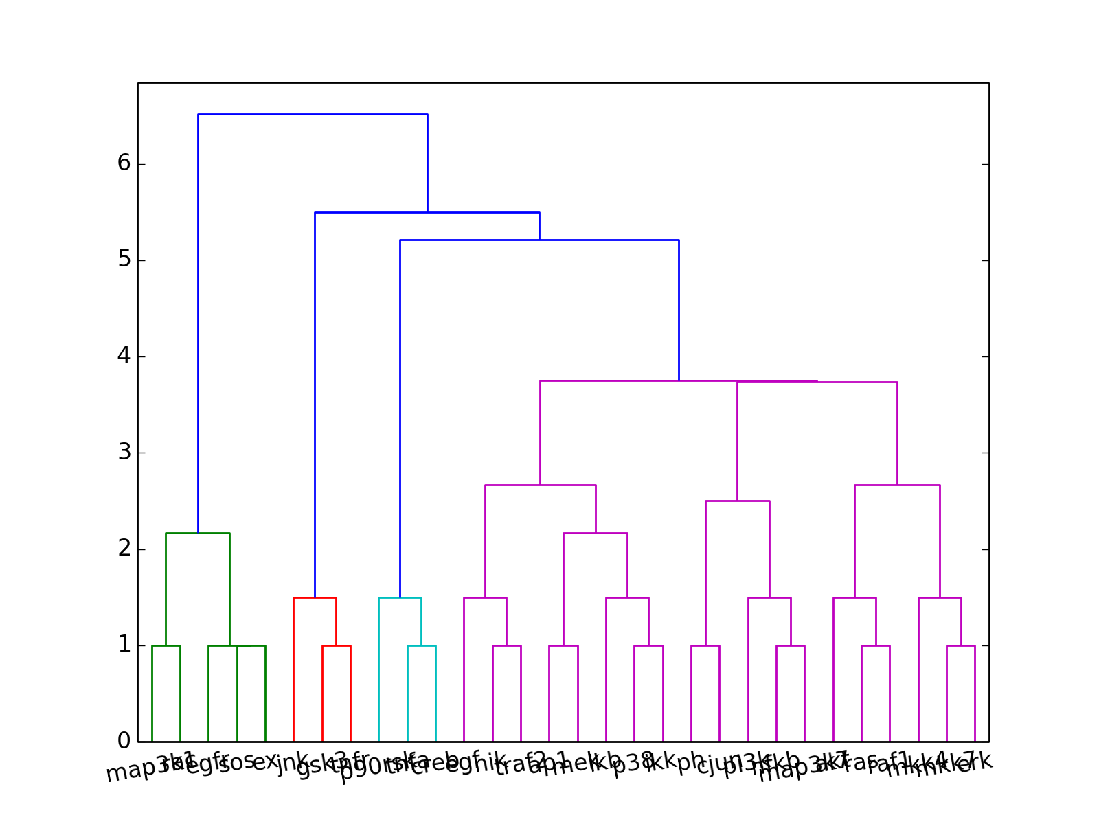
- hcluster()[source]
from cellnopt.core import *
c = CNOGraph(cnodata("PKN-ToyPB.sif"), cnodata("MD-ToyPB.csv"))
c.hcluster()
(Source code, png, hires.png, pdf)

Warning
experimental
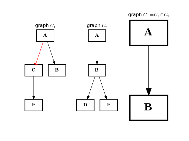
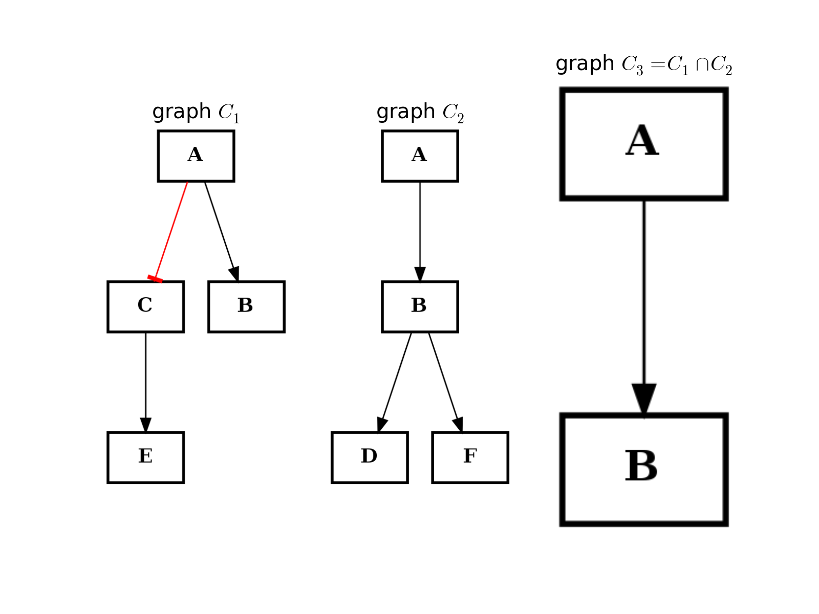
- intersect(other)[source]
Return a graph with only nodes found in “other” graph.
from cellnopt.core import *
from pylab import subplot, title

c1 = CNOGraph()
c1.add_edge("A", "B", link="+")
c1.add_edge("A", "C", link="-")
c1.add_edge("C", "E", link="+")
subplot(1,3,1)
title(r"graph $C_1$")
c1.plotdot(hold=True)

c2 = CNOGraph()
c2.add_edge("A", "B", link="+")
c2.add_edge("B", "D", link="+")
c2.add_edge("B", "F", link="+")
subplot(1,3,2)
c2.plotdot(hold=True)
title(r"graph $C_2$")

c3 = c1.intersect(c2)
subplot(1,3,3)
c3.plotdot(hold=True)
title(r"graph $C_3 = C_1 \cap C_2$")
(Source code, png, hires.png, pdf)

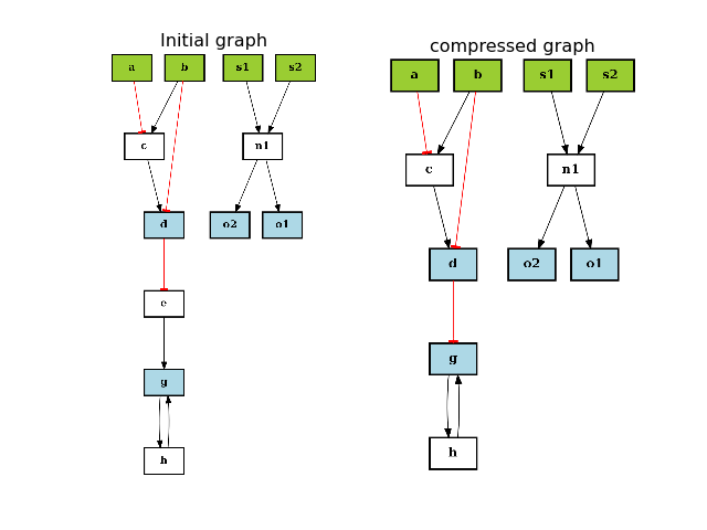
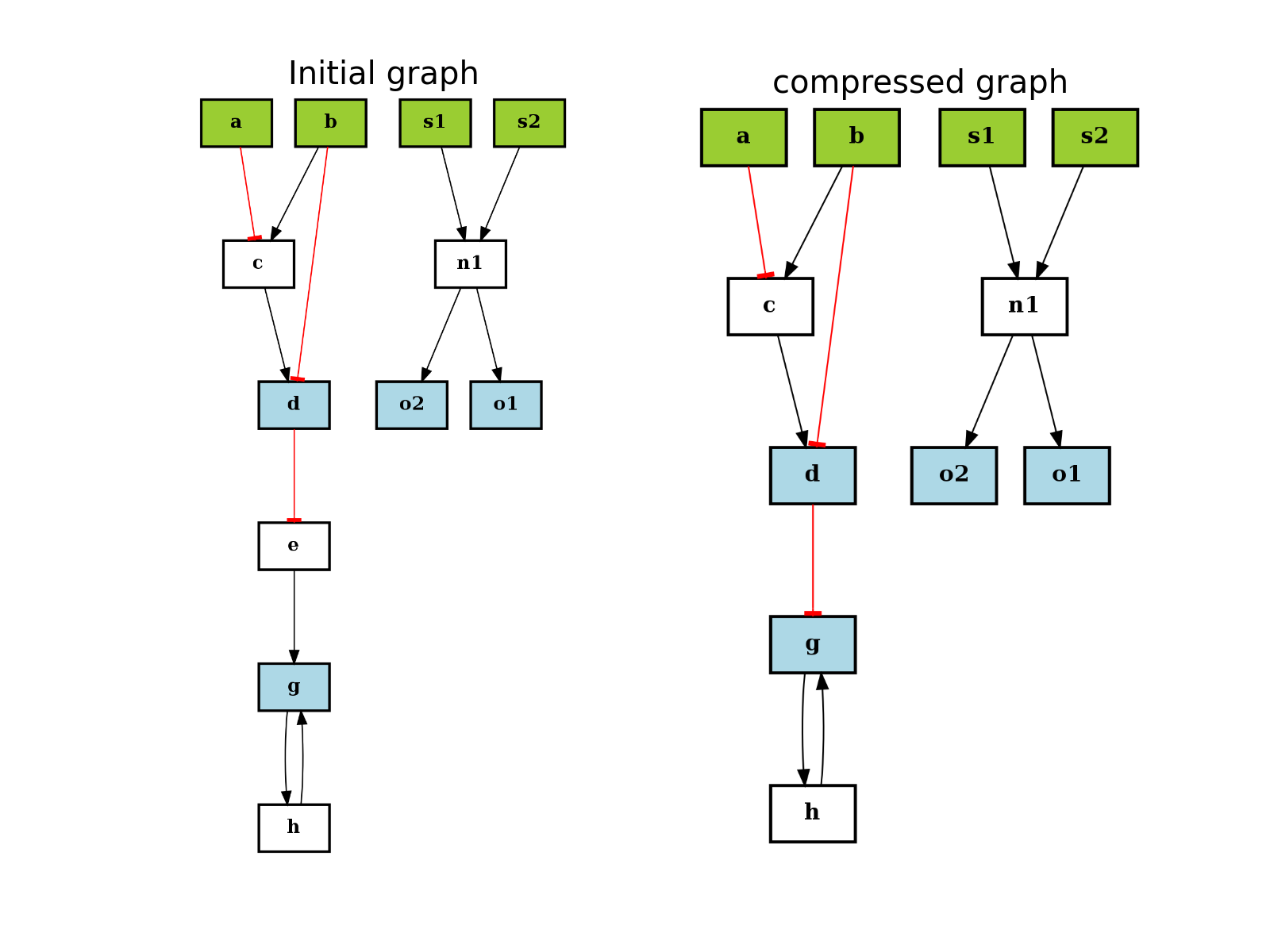
- is_compressable(node)[source]
Returns True if the node can be compressed, False otherwise
Parameters: node (str) – a valid node name Returns: boolean value Here are the rules for compression. The main idea is that a node can be removed if the boolean logic is preserved (i.e. truth table on remaining nodes is preserved).
A node is compressable if it is not part of the stimuli, inhibitors, or signals specified in the MIDAS file.
If a node has several outputs and inputs, it cannot be compressed.
If a node has one input or one output, it may be compressed. However, we must check the following possible ambiguity that could be raised by the removal of the node: once removed, the output of the node may have multiple input edges with different types of inputs edges that has a truth table different from the original truth table. In such case, the node cannot be compressed.
Finally, a node cannot be compressed if one input is also an output (e.g., cycle).
from cellnopt.core import *
from pylab import subplot,show, title
c = cnograph.CNOGraph()
c.add_edge("a", "c", link="-")
c.add_edge("b", "c", link="+")
c.add_edge("c", "d", link="+")
c.add_edge("b", "d", link="-")
c.add_edge("d", "e", link="-")
c.add_edge("e", "g", link="+")
c.add_edge("g", "h", link="+")
c.add_edge("h", "g", link="+")

# multiple inputs/outputs are not removed
c.add_edge("s1", "n1", link="+")
c.add_edge("s2", "n1", link="+")
c.add_edge("n1", "o1", link="+")
c.add_edge("n1", "o2", link="+")

c._stimuli = ["a", "b", "s1", "s2"]
c._signals = ["d", "g", "o1", "o2"]

subplot(1,2,1)
c.plotdot(hold=True)
title("Initial graph")

c.compress()
subplot(1,2,2)
c.plotdot(hold=True)
title("compressed graph")

show()
(Source code, png, hires.png, pdf)
- lookfor(specyName)[source]
Prints information about a species
If not found, try to find species by ignoring cases.
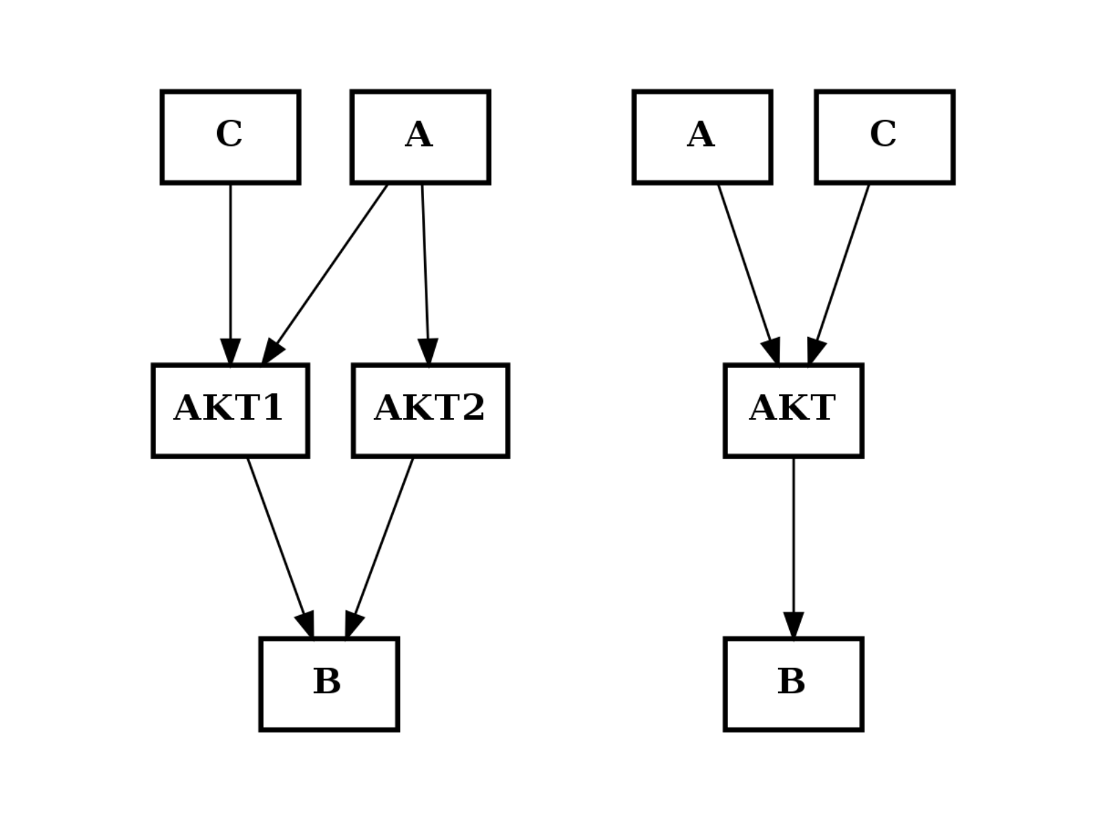
- merge_nodes(nodes, node)[source]
Merge several nodes into a single one
Todo
check that if links of the inputs or outputs are different, there is no ambiguity..
from cellnopt.core import *
from pylab import subplot
c = CNOGraph()
c.add_edge("AKT2", "B", link="+")
c.add_edge("AKT1", "B", link="+")
c.add_edge("A", "AKT2", link="+")
c.add_edge("A", "AKT1", link="+")
c.add_edge("C", "AKT1", link="+")
subplot(1,2,1)
c.plotdot(hold=True)
c.merge_nodes(["AKT1", "AKT2"], "AKT")
subplot(1,2,2)
c.plotdot(hold=True)
(Source code, png, hires.png, pdf)

- midas
MIDAS Read/Write attribute.
- namesSpecies
Return sorted list of species (ignoring and gates) Read-only attribute.
- nonc
Returns list of Non observable and non controlable nodes (Read-only).
- plot(*args, **kargs)[source]
plotting graph using dot program (graphviz) and networkx
By default, a temporary file is created to hold the image created by graphviz, which is them shown using pylab. You can choose not to see the image (show=False) and to save it in a local file instead (set the filename). The output format is PNG. You can play with networkx.write_dot to save the dot and create the SVG yourself.
Parameters: - prog (str) – the graphviz layout algorithm (default is dot)
- viewer – pylab
- legend (bool) – adds a simple legend (default is False)
- show (bool) – show the plot (True by default)
- remove_dot (bool) – if True, remove the temporary dot file.
- edge_attribute_labels – is True, if the label are available, show them. otherwise, if edge_attribute is provided, set lael as the edge_attribute
- aspect – auto or equal. Used to scale the the image (imshow argument) and affects the scaling on the x/y axis.
Additional attributes on the graph itself can be set up by populating the graph attribute with a dictionary called “graph”:
c.graph['graph'] = {"splines":True, "size":(20,20), "dpi":200}
Useful other options are:
c.edge["tnfa"]["tnfr"]["penwidth"] = 3
c.edge["tnfa"]["tnfr"]["label"] = " 5"
If you use edge_attribute and show_edge_labels, label are replaced by the content of edge_attribute. If you still want differnt labels, you must stet show_label_edge to False and set the label attribute manually
c = cnograph.CNOGraph()
c.add_reaction("A=C")
c.add_reaction("B=C")
c.edge['A']['C']['measure'] = 0.5
c.edge['B']['C']['measure'] = 0.1
c.expand_and_gates()
c.edge['A']['C']['label'] = "0.5 seconds"
# compare this that shows only one user-defined label
c.plot()
# with that show all labels
c.plot(edge_attribute="whatever", edge_attribute_labels=False)
See the graphviz homepage documentation for more options.
Note
edge attribute in CNOGraph (Directed Graph) are not coded in the same way in CNOGraphMultiEdges (Multi Directed Graph). So, this function does not work for MultiGraph
Todo
use same colorbar as in midas. rigtht now; the vmax is not correct.
Todo
precision on edge_attribute to 2 digits.
- plotdot(prog='dot', viewer='pylab', hold=False, legend=False, show=True, filename=None, node_attribute=None, edge_attribute=None, cmap=None, colorbar=False, remove_dot=True, cluster_stimuli=False, normalise_cmap=True, edge_attribute_labels=True, aspect='equal', rank=False)[source]
plotting graph using dot program (graphviz) and networkx
By default, a temporary file is created to hold the image created by graphviz, which is them shown using pylab. You can choose not to see the image (show=False) and to save it in a local file instead (set the filename). The output format is PNG. You can play with networkx.write_dot to save the dot and create the SVG yourself.
Parameters: - prog (str) – the graphviz layout algorithm (default is dot)
- viewer – pylab
- legend (bool) – adds a simple legend (default is False)
- show (bool) – show the plot (True by default)
- remove_dot (bool) – if True, remove the temporary dot file.
- edge_attribute_labels – is True, if the label are available, show them. otherwise, if edge_attribute is provided, set lael as the edge_attribute
- aspect – auto or equal. Used to scale the the image (imshow argument) and affects the scaling on the x/y axis.
Additional attributes on the graph itself can be set up by populating the graph attribute with a dictionary called “graph”:
c.graph['graph'] = {"splines":True, "size":(20,20), "dpi":200}
Useful other options are:
c.edge["tnfa"]["tnfr"]["penwidth"] = 3
c.edge["tnfa"]["tnfr"]["label"] = " 5"
If you use edge_attribute and show_edge_labels, label are replaced by the content of edge_attribute. If you still want differnt labels, you must stet show_label_edge to False and set the label attribute manually
c = cnograph.CNOGraph()
c.add_reaction("A=C")
c.add_reaction("B=C")
c.edge['A']['C']['measure'] = 0.5
c.edge['B']['C']['measure'] = 0.1
c.expand_and_gates()
c.edge['A']['C']['label'] = "0.5 seconds"
# compare this that shows only one user-defined label
c.plot()
# with that show all labels
c.plot(edge_attribute="whatever", edge_attribute_labels=False)
See the graphviz homepage documentation for more options.
Note
edge attribute in CNOGraph (Directed Graph) are not coded in the same way in CNOGraphMultiEdges (Multi Directed Graph). So, this function does not work for MultiGraph
Todo
use same colorbar as in midas. rigtht now; the vmax is not correct.
Todo
precision on edge_attribute to 2 digits.
- preprocessing(expansion=True, compression=True, cutnonc=True, maxInputsPerGate=2)[source]
Performs the 3 preprocessing steps (cutnonc, expansion, compression)
Parameters: - expansion (bool) – calls expand_and_gates() method
- compression (bool) – calls compress() method
- cutnon (bool) – calls cutnonc() method
- maxInputPerGates (int) – parameter for the expansion step
from cellnopt.core import *
c = CNOGraph(cnodata("PKN-ToyPB.sif"), cnodata("MD-ToyPB.csv"))
c.preprocessing()
c.plotdot()
(Source code, png, hires.png, pdf)

- reacID
return the reactions (edges)
- recursive_compress(max_num_iter=25)[source]
Recursive compression.
Sometimes, when networks are large and complex, calling the compress() only once may not be enough to remove all compressable nodes. Calling this function guarantees that all compressable nodes are removed.
- relabel_nodes(mapping)[source]
see rename_node()
- remove_and_gates()[source]
Remove the AND nodes added by expand_and_gates()
- remove_edge(u, v)[source]
Remove the edge between u and v.
Parameters: - u (str) – node u
- u – node v
Calls clean_orphan_ands() afterwards
- remove_node(n)[source]
Remove a node n
Parameters: node (str) – the node to be removed Edges linked to n are also removed. AND gate may now be irrelevant (only one input or no input). Orphan AND gates are removed.
See also
- remove_nodes_from(nbunch)[source]
Removes a bunch of nodes
Warning
need to be tests with and gates.
- rename_node(mapping)[source]
Function to rename a node, while keeping all its attributes.
Parameters: mapping (dict) – a dictionary mapping old names (keys) to new names (values ) Returns: new cnograph object if we take this example:
c = CNOGraph();
c.add_reaction("a=b");
c.add_reaction("a=c");
c.add_reaction("b=d");
c.add_reaction("c=d");
c.expand_and_gates()
Here, an AND gate has been created. c.nodes() tells us that its name is “b^c=d”. If we rename the node b to blong, the AND gate name is unchanged if we use the nx.relabel_nodes function. Visually, it is correct but internally, the “b^c=d” has no more meaning since the node “b” does not exist anymore. This may lead to further issues if we for instance split the node c:
c = nx.relabel_nodes(c, {"b": "blong"})
c.split_node("c", ["c1", "c2"])
This function calls relabel_node taking care of the AND nodes as well.
Warning
this is not inplace modifications.
- reset_edge_attributes()[source]
set all edge attributes to default attributes
See also
set_default_edge_attribute()
if we set an edge label, which is an AND ^, then plot fails in this function c.edge[“alpha^NaCl=HOG1”][‘label’] = ”?”
- sif()[source]
Return a SIF instance corresponding to this graph
Warning
need to fix the reacID attribute to get AND gates
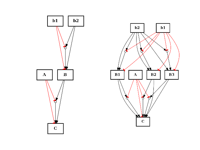
- split_node(node, nodes)[source]
from cellnopt.core import *
from pylab import subplot
c = CNOGraph()
c.add_reaction("!A=C")
c.add_reaction("B=C")
c.add_reaction("!b1=B")
c.add_reaction("b2=B")
c.expand_and_gates()

subplot(1,2,1)
c.plotdot(hold=True)

c.split_node("B", ["B1", "B2", "B3"])
subplot(1,2,2)
c.plotdot(hold=True)
(Source code, png, hires.png, pdf)

- swap_edges(nswap=1)[source]
Swap two edges in the graph while keeping the node degrees fixed.
A double-edge swap removes two randomly chosen edges u-v and x-y and creates the new edges u-x and v-y:
u--v                u  v
        becomes     |  |
x--y                x  y
If either the edge u- x or v-y already exist no swap is performed and another attempt is made to find a suitable edge pair.
Parameters: nswap (int) – number of swaps to perform (Defaults to 1) Returns: nothing Warning
the graph is modified in place.
Todo
need to take into account the AND gates !!
a proposal swap is ignored in 3 cases: #. if the summation of in_degree is changed #. if the summation of out_degree is changed #. if resulting graph is disconnected
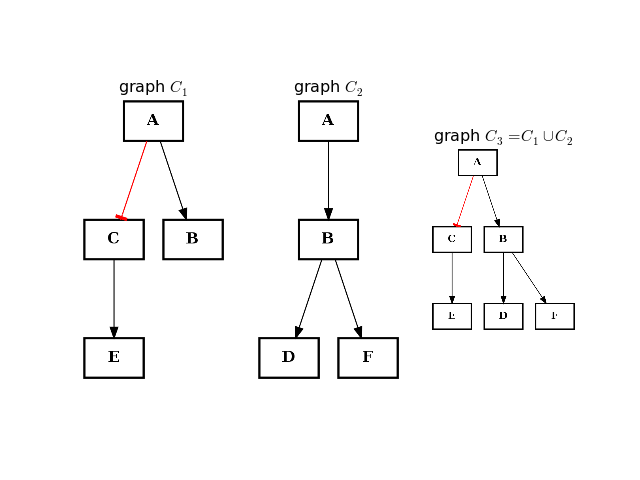
- union(other)[source]
Return graph with elements from this instance and the input graph.
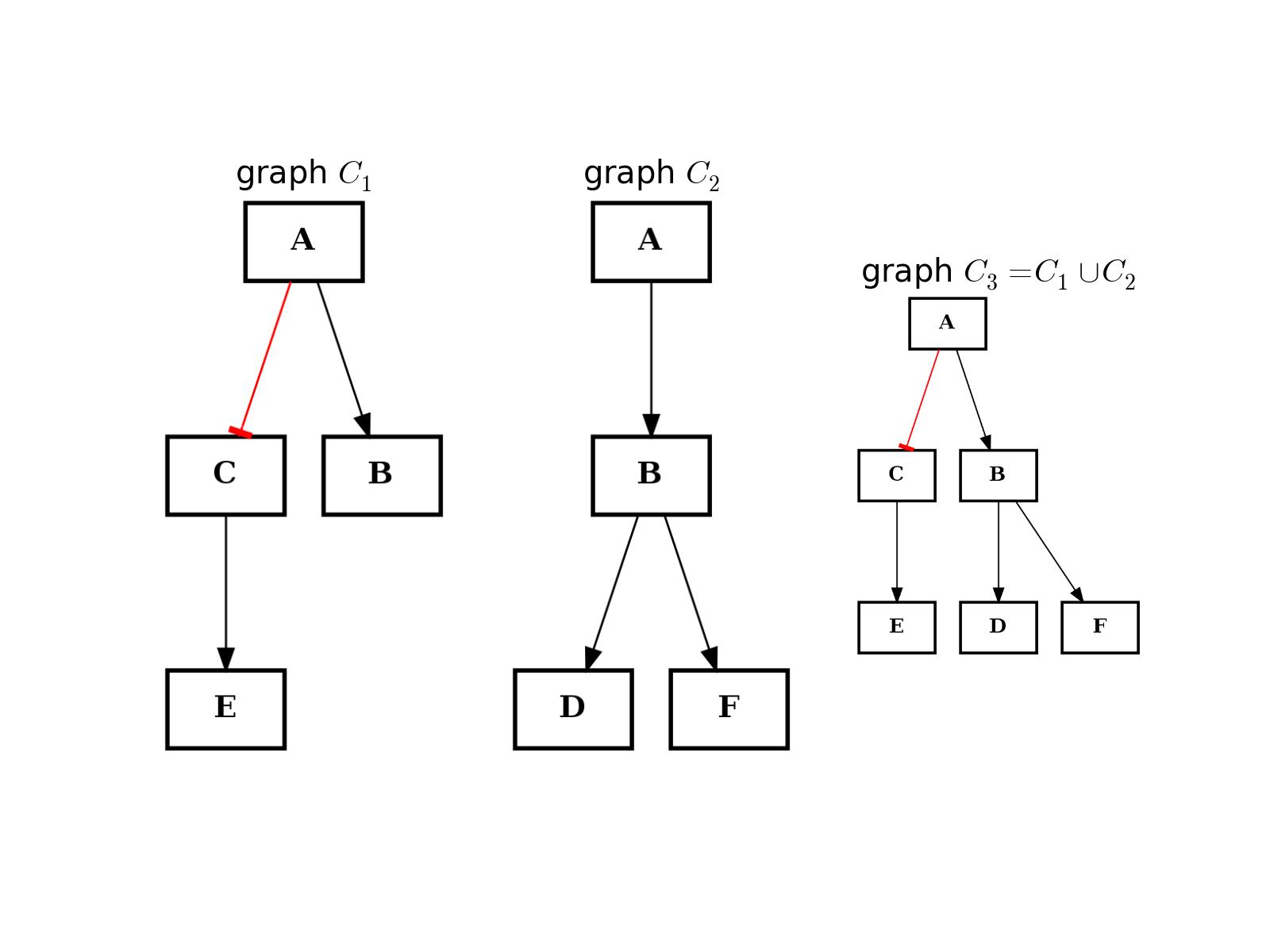
from cellnopt.core import *
from pylab import subplot, title

c1 = CNOGraph()
c1.add_edge("A", "B", link="+")
c1.add_edge("A", "C", link="-")
c1.add_edge("C", "E", link="+")
subplot(1,3,1)
title(r"graph $C_1$")
c1.plotdot(hold=True)

c2 = CNOGraph()
c2.add_edge("A", "B", link="+")
c2.add_edge("B", "D", link="+")
c2.add_edge("B", "F", link="+")
subplot(1,3,2)
c2.plotdot(hold=True)
title(r"graph $C_2$")

c3 = c1.union(c2)
subplot(1,3,3)
c3.plotdot(hold=True)
title(r"graph $C_3 = C_1 \cup C_2$")
(Source code, png, hires.png, pdf)
- class CNOGraphMultiEdges(model=None, data=None, verbose=False, **kargs)[source]
A multiDigraph version of CNOGraph.
Warning
experimental
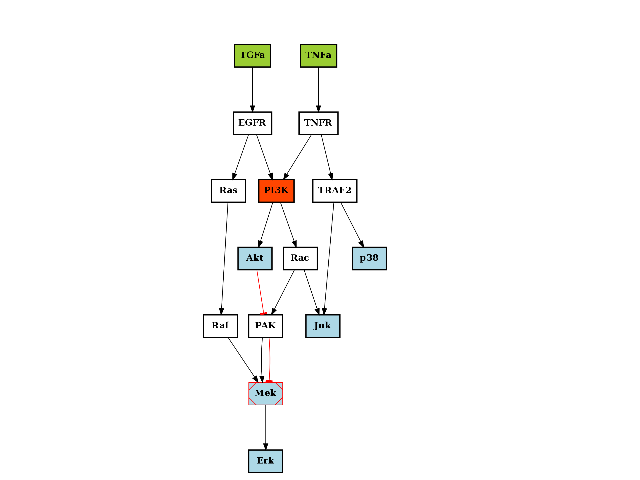
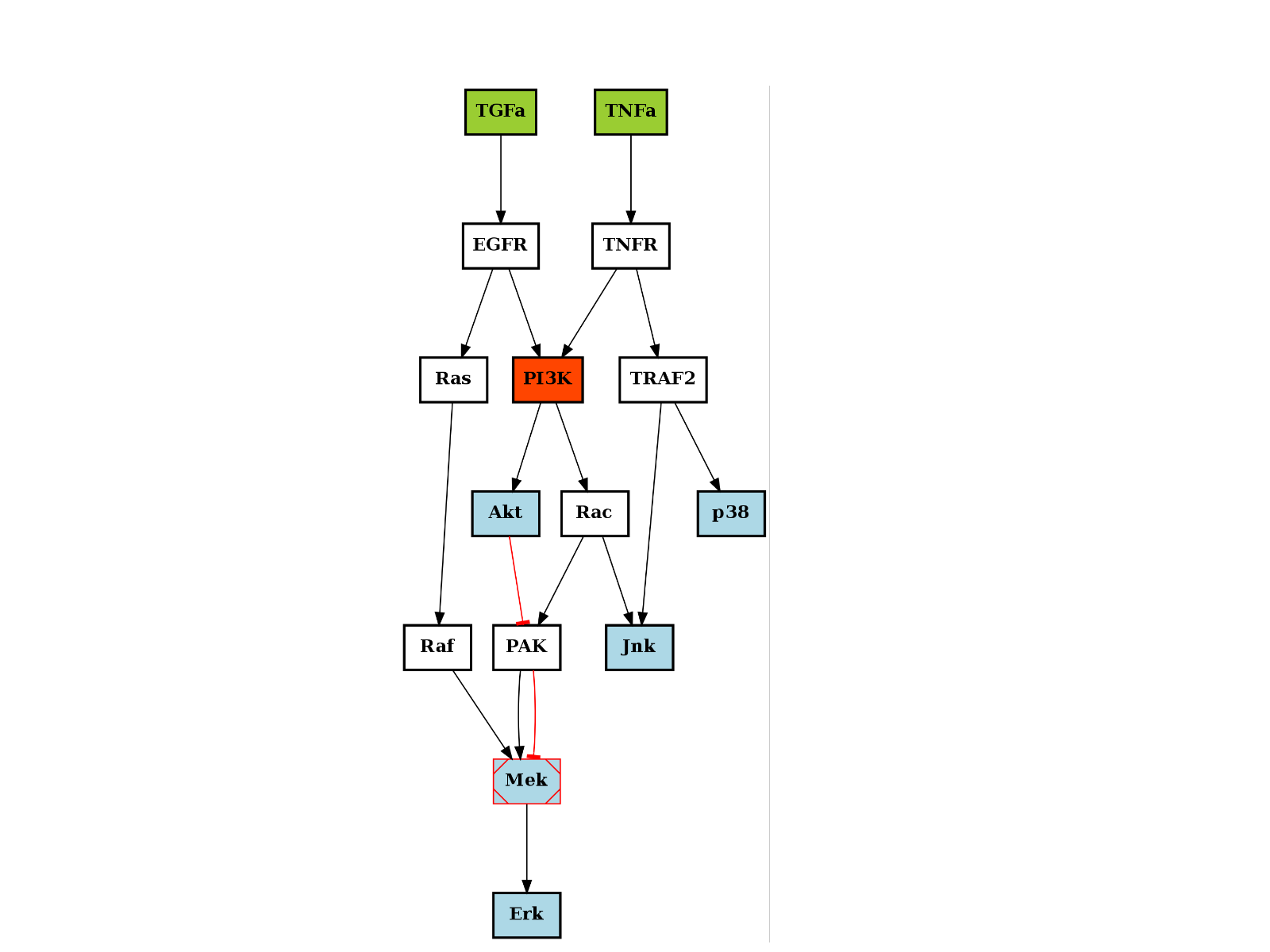
>>> from cellnopt.core import *
>>> c = cnograph.CNOGraphMultiEdges(cnodata("PKN-ToyPCB.sif"), cnodata("MD-ToyPCB.csv"))
>>> c.add_edge("PAK", "Mek", link="-")
>>> c.plot()
(Source code, png, hires.png, pdf)
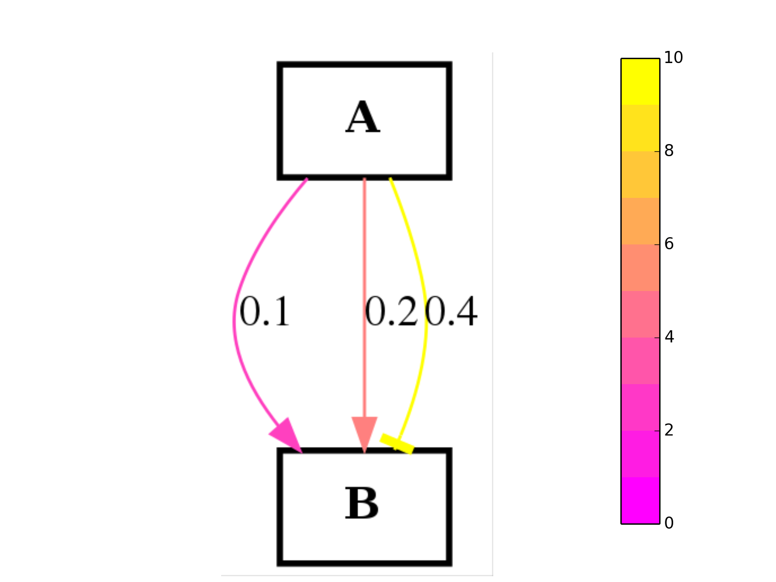
>>> from cellnopt.core import *
>>> c2 = cnograph.CNOGraphMultiEdges()
>>> c2.add_edge("A","B", link="+", edgecolor=.1)
>>> c2.add_edge("A","B", link="+", edgecolor=.2)
>>> c2.add_edge("A","B", link="-", edgecolor=.3)
>>> c2.add_edge("A","B", link="-", edgecolor=.4)
>>> c2.plot(edge_attribute="edgecolor", colorbar=True, cmap="spring")
(Source code, png, hires.png, pdf)

Todo
self.reacID attribute does not work
- compressable_nodes
- remove_edge(u, v, key=None)[source]
Remove the edge between u and v.
Parameters: - u (str) – node u
- u – node v
Calls clean_orphan_ands() afterwards
1.2. MIDAS related
1.2.1. MIDAS
- class XMIDAS(filename=None, cellLine=None, verbose=False)[source]
XMIDAS dat structure. X stands for extended and replaces MIDASReader class.
from cellnopt.core import XMIDAS
m = XMIDAS(cnodata("tes.csv"))
m.df # access to the data frame
m.scale_max(gain=0.9)   # scale over all experiments and time finding the max
                # and scaling (divide by max) for each species individually.
m.corr()        # alias to m.df.corr() removing times/experiments
columns


tuples = [(exp, time) for exp in ["exp1", "exp2"] for time in [0,1,2,3,4]]
index = pd.MultiIndex.from_tuples(tuples, names=["experiment", "time"])
xx = pd.DataFrame(randn(10,2), index=index, columns=["Akt", "Erk"])
What remains to be done ?
- average over celltypes To be done in MultiMIDAS
Warning
if there are replicates, call average_replicates before creating a simulation or calling plot”mode=”mse”)
Todo
when using MSE, an option could be to average the errors by taking into account the time. In other words, a weight/integral. if t = 1,2,3,4,5,10,60, the errors on 1,2,3,4,5 are more important than between 5,10,60. does it make sense ?
Todo
make df a property to handle sim properly, if not scaled, sim and exp seems to have the same scale also errors are large as expected
Warning
MD-TR-33333-JITcellData.csv contains extra ,,,, at the end. should be removed or ignored
Todo
colorbar issue with midas.XMIDAS(“share/data/MD-test_4andgates.csv”)
Todo
when plotting, if there is only 1 stimuli and 5-6 inhibitors, the width of the stimuli is the same as the one with the inhibitors. cell size should be identical, not stretched. See e..g., “EGFR-ErbB_PCB2009.csv”
Todo
when ploting the mse, we should be able to plotonly a subset of the time indices (useful for bollean analysis at a given time)
..todo:: a MIDAS class to check validity just to simplfy the XMIDAs class itself.
Todo
inhibitors ends in :i to avoid clashes with same name in stimuli..
- add_gaussian_noise(sigma=0.1, inplace=False)[source]
add gaussian noise to the data. Results may be negative or above 1
- add_uniform_distributed_noise(inplace=False, dynamic_range=1, mode=u'bounded')[source]
add random (uniformaly distributed) noise to the dataframe
The noise is uniformliy distributed between -0.5 and 0.5 and added to the values contained in the dataframe (for each combinaison of species and time/experiment). New values are
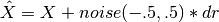 ,
where dr is the dynamical range. Note that final values may be below
zero or above 1. If you do not want this feature, set the mode to
“bounded” (The default is free). bounded mens
,
where dr is the dynamical range. Note that final values may be below
zero or above 1. If you do not want this feature, set the mode to
“bounded” (The default is free). bounded mensParameters: - inplace (bool) – False by default
- dynamic_range (float) – a multiplicative value set to the noise
- min_value (bool) – final values below min are set to min (default is 0)
- max_value (bool) – final values above max are set to max (default is 1)
- cellLine
- cellLines
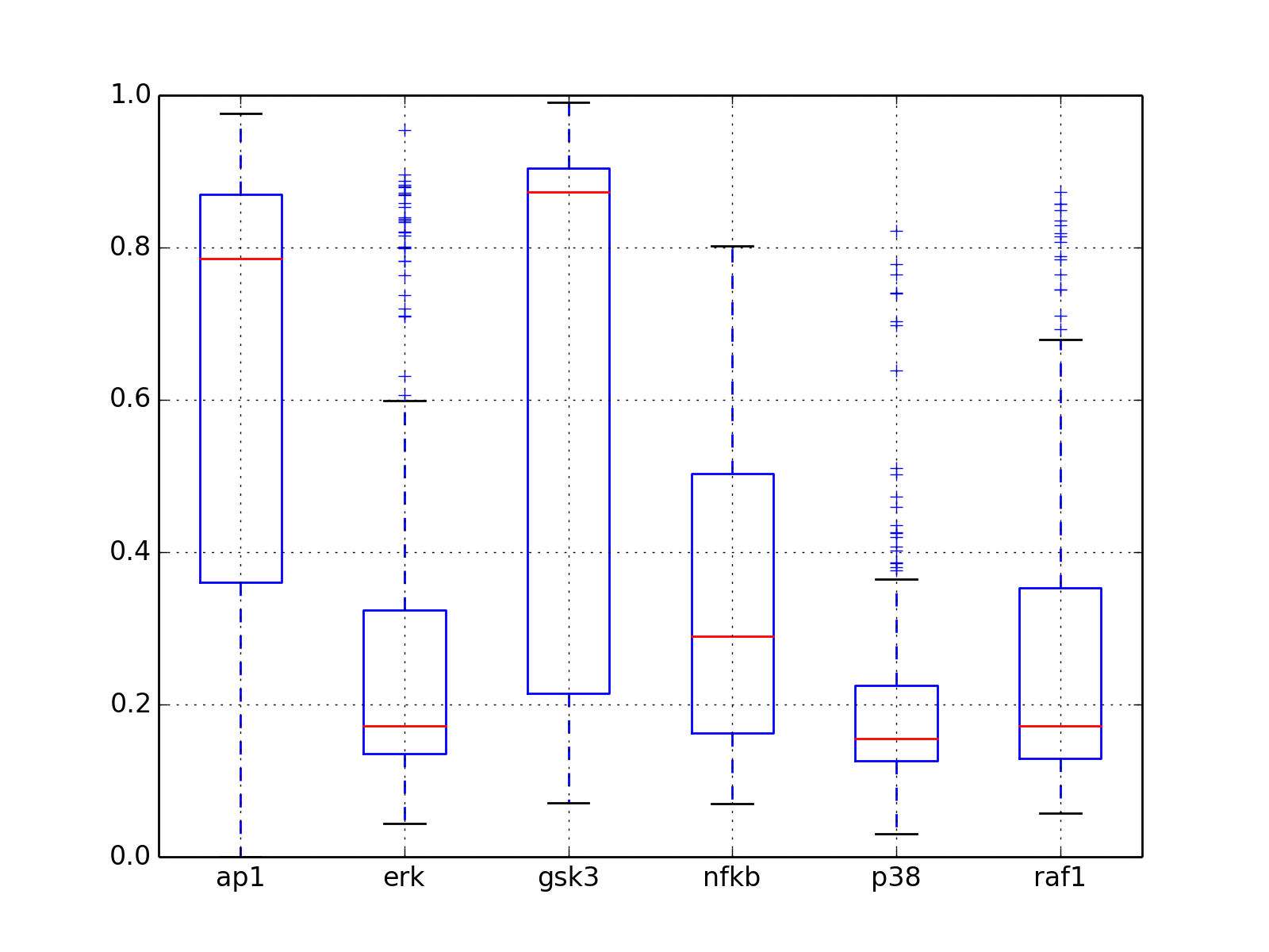
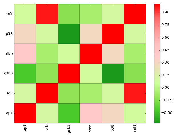
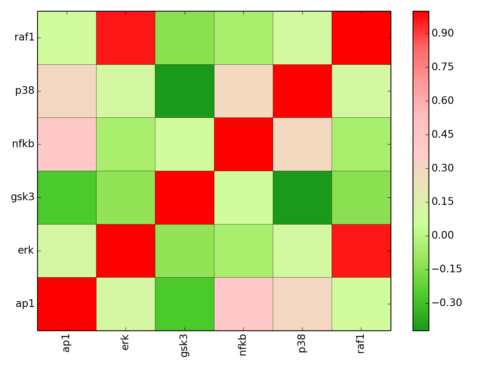
- corr(names=None, cmap=None)[source]
plot correlation between the measured species
Parameters: - names (list) – restriction to some species if provided.
- cmap (string) – a valid colormap (e.g. jet). Can also use “green” or “heat”.
>>> from cellnopt.core import *
>>> m = XMIDAS(cnodata("MD-ToyPB.csv"))
>>> m.corr(cmap="green")
(Source code, png, hires.png, pdf)

- create_empty_simulation()[source]
Populate the simulation dataframe with zeros.
The simulation has the same layout as the experiment.
The dataframe is stored in sim.
- create_random_simulation()[source]
Populate the simulation dataframe with uniformly random values.
The simulation has the same layout as the experiment.
The dataframe is stored in sim.
- discretise(inplace=True, N=2)[source]
Parameters: - N (int) – number of discrete values (defaults to 2). If set to 2, values will be either 0 or 1. If set to 5, values wil lbe in [0,0.25,0.5,0.75,1]
- inplace –
- experiments
Return dataframe with experiments
- export2experiments()[source]
Returns list of Experiments
Each datum in the dataframe df is converted into an instance of Experiment.
Returns: list of experiments. Todo
use Experiments
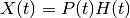
- get_diff(sim=None, norm=u'square', normed=True)[source]
return difference between X and simulation. Take absolute. if norm == square or norm == absolute takes absolute values. if norm == square, also take power of 2.
divide by number of time points.
Todo
doc
- get_residual_errors(level=u'time', normed=False)[source]
Return vector with residuals errors
The residual errors are interesting to look at in the context of a boolean analysis. Indeed, residual errors is the minimum error that is unavoidable with a boolean network and comes from the discrete nature of such a model. In a boolean analysis, one would compare 0/1 values to continuous values between 0 and 1. Therefore, however good is the optimisation, the value of the goodness of fit term cannot go under this residual error.
Param: level to sum over. Returns: returns residual errors 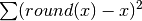 the summation is performed over species and experiment by default
>>> from cellnopt.core import cnodata, XMIDAS
>>> m = XMIDAS(cnodata("MD-ToyMMB_T2.csv"))
>>> m.get_residual_errors()
time
0       0.000000
10      2.768152
100     0.954000
dtype: float64
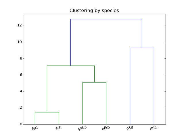
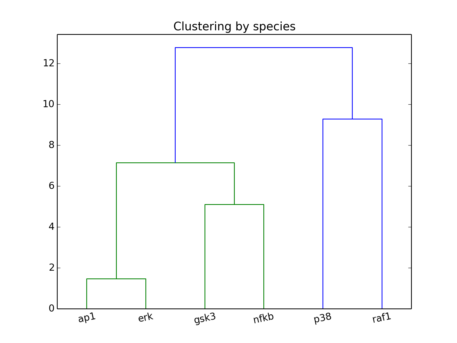
- hcluster(mode=u'experiment')[source]
from cellnopt.core import *
m = midas.XMIDAS(cnodata("MD-ToyPB.csv"))
m.hcluster("species")
(Source code, png, hires.png, pdf)
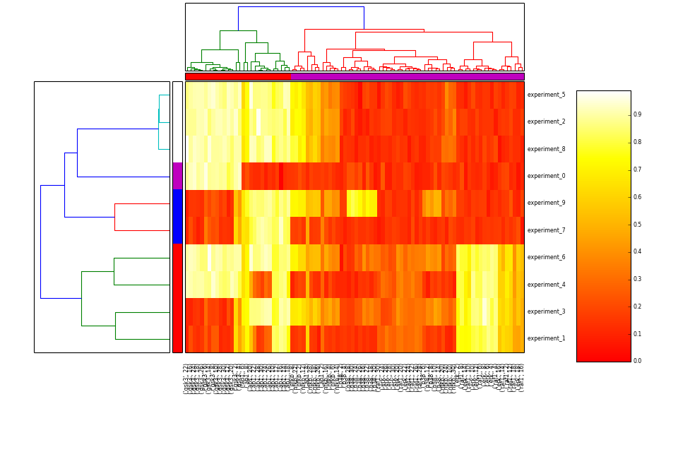
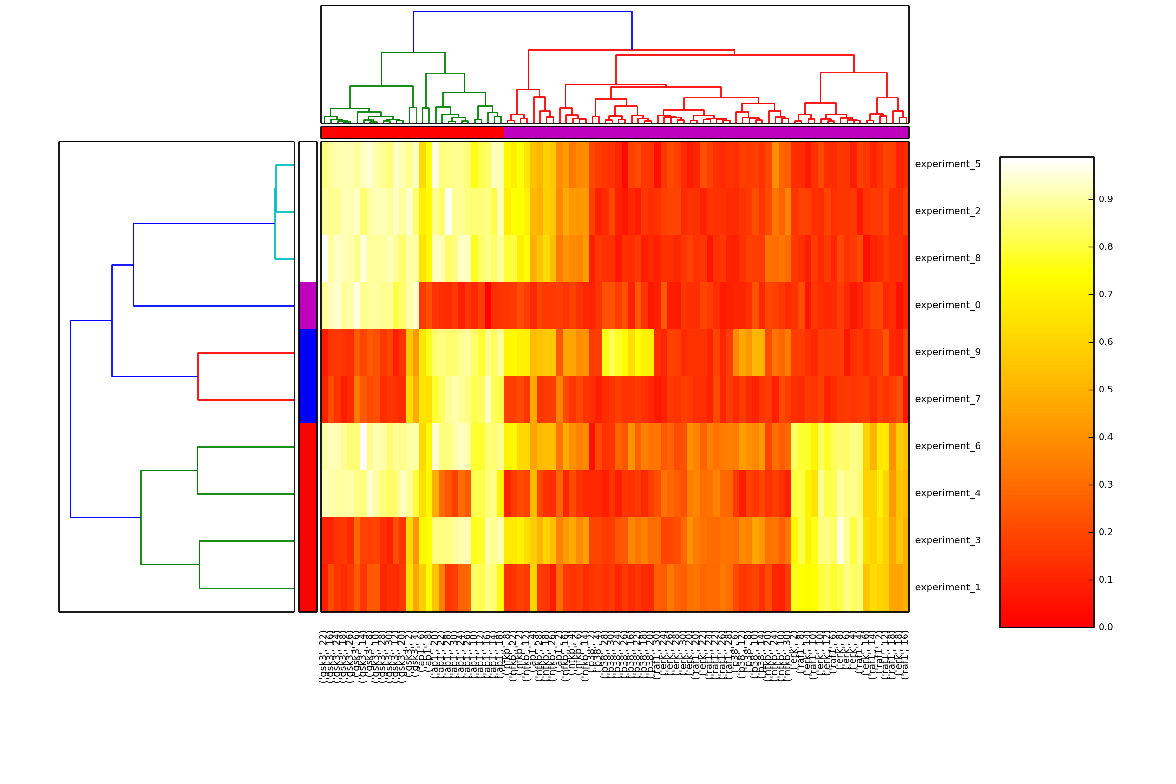
- heatmap(cmap=u'heat', transpose=False)[source]
Hierarchical clustering on species and one of experiment/time level
from cellnopt.core import *
m = midas.XMIDAS(cnodata("MD-ToyPB.csv"))
m.heatmap()
(Source code, png, hires.png, pdf)

- inhibitors
return the inhibitors dataframe
- nExps
return number of experiments
- nSignals
return the number of signals
- names_cues
Return list of stimuli and inhibitors together
- names_inhibitors
- names_signals
same as names_species
- names_species
list of species
- names_stimuli
- normalise(mode, inplace=True, changeThreshold=0, **kargs)[source]
Normalise the data
Parameters: - mode – time or controle
- inplace (bool) – Defaults to True.
see normalise.XMIDASNormalise
Warning
not fully tested. the mode “time” should work. The control mode has been tested on 2 MIDAS file only.
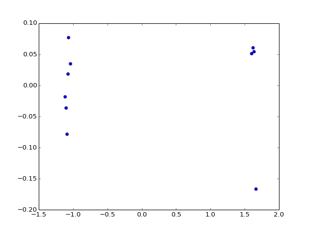
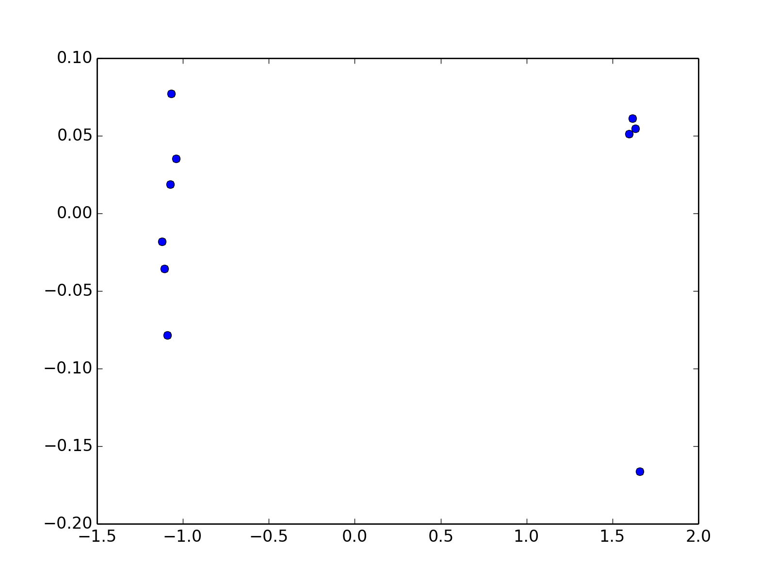
- pca(signal, pca_components=2)[source]
Not sure this is the proper way...
get all experiment related to 1 signal
from cellnopt.core import *
m = midas.XMIDAS(cnodata("MD-ToyPB.csv"))
#m.df = abs(m.df)
#m.df/=m.df.max()
m.pca("gsk3")
(Source code, png, hires.png, pdf)

Todo
pls = PLSRegression(n_components=3) from sklearn.pls import PLSCanonical, PLSRegression
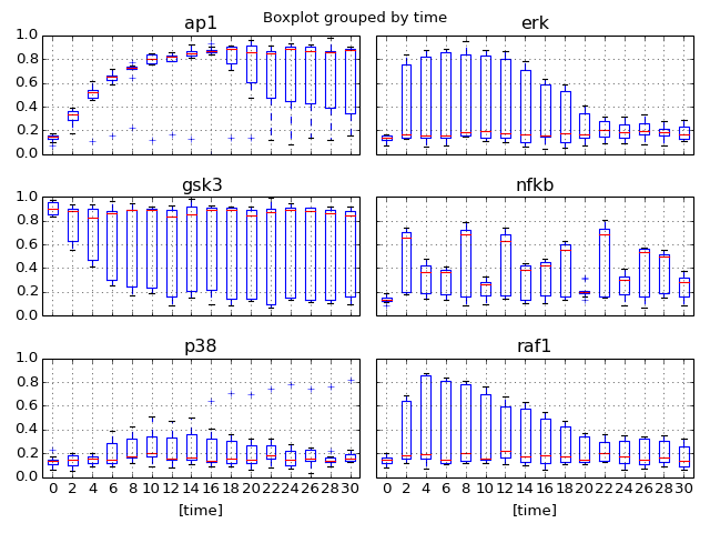
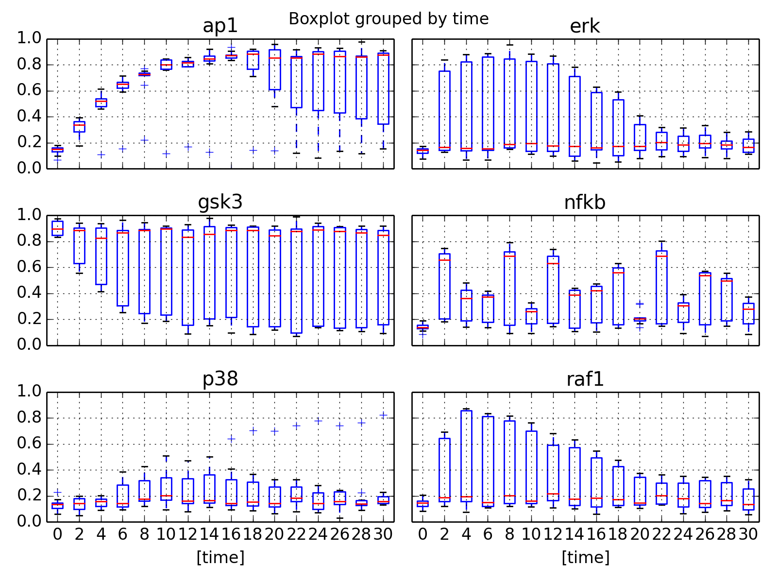
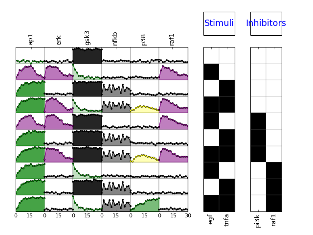
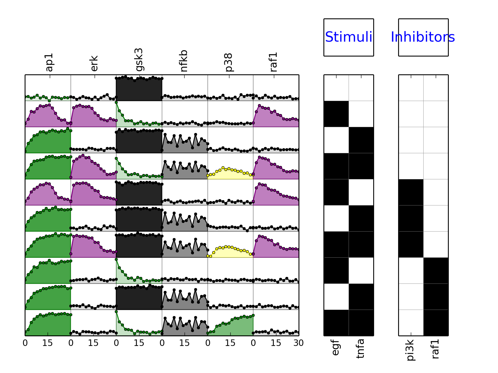
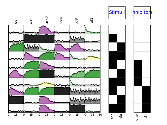
- plot(**kargs)[source]
Parameters: mode (string) – must be either “mse” or “trend” (defaults to trend) calls plotMSEs and plotExp
if mode == mse, calls also plotSim
from cellnopt.core import *
m = XMIDAS(cnodata("MD-ToyPB.csv"))
m.plot(mode="trend")
(Source code, png, hires.png, pdf)

Todo
a zero line
- plotExp(markersize=3, logx=False, color=u'black', **kargs)[source]
plot experimental curves
>>> from cellnopt.core import *
>>> m = midas.MIDASReader(cnodata("MD-ToyPB.csv"));
>>> m.plotMSEs()
>>> m.plotExp()
Note
called by plot()
See also
- plotMSEs(cmap=u'heat', N=10, norm=u'square', rotation=90, margin=0.05, colorbar=True, vmax=None, vmin=0.0, mode=u'trend', **kargs)[source]
plot MSE errors and layout
>>> from cellnopt.core import *
>>> m = midas.MIDASReader(cnodata("MD-ToyPB.csv"));
>>> m.plotMSEs()
Todo
error bars
Todo
dynamic fontsize in the signal names ?
Note
called by plot()
See also
Todo
need to make it more modular e.g. no cues matrices
- plotSim(markersize=3, logx=False, linestyle=u'--', lw=1, color=u'b', marker=u'x', **kargs)[source]
plot experimental curves
>>> from cellnopt.core import *
>>> m = midas.MIDASReader(cnodata("MD-ToyPB.csv"));
>>> m.plotMSEs()
>>> m.plotExp()
>>> m.plotSim()
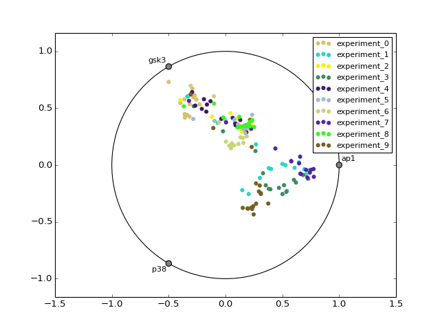
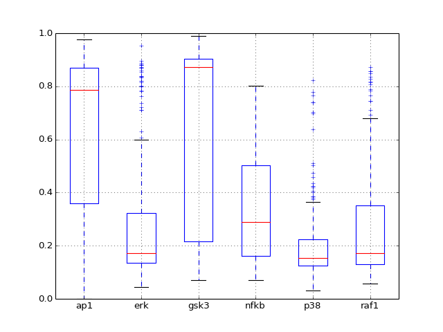
- radviz(species=None, fontsize=10)[source]
from cellnopt.core import *
m = XMIDAS(cnodata("MD-ToyPB.csv"))
m.radviz(["ap1", "gsk3", "p38"])
(Source code, png, hires.png, pdf)
- remove_cellLine(labels)[source]
Remove a cellLine from the dataframe.
Does not really work since there is only one cellLine in the dataframe. all data is contained in data but the current dataframe contains only one, which can be changed simply by setting the cellLine attribute with one of the valid cellLine found in the cellLines attribute
- remove_experiments(labels)[source]
Remove experiment(s) from the dataframe
Parameters: labels (list) – one experiment or a list of experiments. Valid experiments are in the experiments.index dataframe. Experiments are of the form “experiment_12”. You can refer to an experiment by its number (e.g., here 12).
- remove_inhibitors(labels)[source]
Remove inhibitor(s) from the experiment dataframe
Parameters: labels – a string or list of string representing the inhibitor(s)
- remove_species(labels)[source]
Remove a set of species
Parameters: labels – list of Species (list of strings) or just one species(single string or as a list. m.remove_species("p38") m.remove_species(["p38"])
- remove_stimuli(labels)[source]
Remove a stimuli from the experiment dataframe
Parameters: labels – a string or list of string representing the stimuli
- remove_times(labels)[source]
Remove time values from the data
Parameters: labels (list) – one time point or a list of time points. Valid time points are in the times attribute.
- rename_cellLine(to_replace)[source]
Rename cellLine indices
Parameters: to_replace (dict) – dictionary with mapping of values to be replaced. For example; to convert time in minutes to time in seconds, use something like:
m.rename_cellLine({"undefined": "PriHu"})
- rename_inhibitors(names_dict)[source]
Rename inhibitors
Parameters: names_dict – a dictionary with names (keys) to be replaced (values) from cellnopt.core import * m = XMIDAS(cnodata("MD-ToyPB.csv")) m.rename_species({"raf:i":"RAF:i"})
See also
Warning
inhibitor name must end with the string :i
Todo
sanity check that the pair of key/value contain the :i characters
- rename_species(names_dict)[source]
Rename species in the main df dataframe
Parameters: names_dict – a dictionary with names (keys) to be replaced (values) from cellnopt.core import * m = XMIDAS(cnodata("MD-ToyPB.csv")) m.rename_species({"erk":"ERK", "akt":"AKT"})
See also
- rename_stimuli(names_dict)[source]
Rename stimuli in the experiment dataframe
Parameters: names_dict – a dictionary with names (keys) to be replaced (values) from cellnopt.core import * m = XMIDAS(cnodata("MD-ToyPB.csv")) m.rename_species({"erk":"ERK", "akt":"AKT"})
See also
- rename_time(to_replace)[source]
Rename time indices
Parameters: to_replace (dict) – dictionary with mapping of values to be replaced. For example; to convert time in minutes to time in seconds, use something like:
m.rename_time({0:0,1:1*60,5:5*60})
- reset_index()[source]
Remove all indices (cellLine, time, experiment)
Done in the 3 dataframes df, sim and errors
- save2midas(filename, expand_time_column=False)[source]
Save XMIDAS into a MIDAS CSV file.
Parameters: filename (str) –
- scale_max_across_experiments(inplace=True)[source]
Divide each species column by max acrosss all experiments
In the MIDAS plot, this is equivalent to dividig each column by the max over that column. So, on each column, you should get 1 max values set to 1 (if the max is unique). The minimum values may not be set to 0.
- scale_min_max(inplace=True)[source]
Divide all data by the maximum over entire data set
where
 and
and  ,
with
,
with  the experiment, with
  the species,
with
the species,
with  the time.
- scale_min_max_across_experiments(inplace=True)[source]
Rescale each species column across all experiments
- set_index()[source]
Reset all indices (cellLine, time, experiment)
Done in the 3 dataframes df, sim and errors
- shuffle(mode=u'experiment', inplace=True)[source]
Shuffle data
Parameters: mode (str) – timeseries shuffles experiments and species; timeseries are unchanged. all shuflles through time, experiment and species. mode can be
# timeseries that is # all # signals or species: sum over signals is constant
- by_signals (or by_species, by_columns, species, signals,
columns) shuffles each column independently. All values are shuffled but the sum over a column/species remains identical. constqnt is df.sum()
- # shuffle over index. This means that values with same cell/exp/time are shuffled;
- This is therefore over species as well but keep a kind of time information constqnt is sum over experiment: m.df.sum(level=”experiment”).sum(axis=1)
(Source code, png, hires.png, pdf)

Shuffling qll timeseries keeping their structures:
from cellnopt.core import *
m = midas.XMIDAS(cnodata("MD-ToyPB.csv"))
m.shuffle(mode="timeseries")
m.plot()
(Source code, png, hires.png, pdf)

- signals
Getter for the columns of the dataframe that represents the species/signals
- species
Getter for the columns of the dataframe that represents the species/signals
- stimuli
return the stimuli dataframe
- times

- class MultiMIDAS(filename=None)[source]
Data structure to store multiple instances of MIDAS files
You can read a MIDAS file that contains several cell lines: and acces to the midas files usig their cell line name
>>> mm = MultiMIDAS(cnodata("EGFR-ErbB_PCB2009.csv"))
>>> mm.cellLines
['HepG2', 'PriHu']
>>> mm["HepG2"].namesCues
['TGFa', 'MEK12', 'p38', 'PI3K', 'mTORrap', 'GSK3', 'JNK']
where the list of cell line names is available in the cellLines attribute.
Or you can start from an empty list and add instance later on using addMIDAS() method.
constructor
Parameters: filename (str) – a valid MIDAS file (optional) - addMIDAS(midas)[source]
Add an existing MIDAS instance to the list of MIDAS instances
>>> from cellnopt.core import *
>>> m = MIDASReader(cnodata("MD-ToyPB.csv"))
>>> mm = MultiMIDAS()
>>> mm.addMIDAS(m)
- cellLines
return names of all cell lines, which are the MIDAS instance identifier
- plot()[source]
Call plot() method for each MIDAS instances in different figures
More sophisticated plots to easily compare cellLines could be implemented.
- readMIDAS(filename)[source]
read MIDAS file and extract individual cellType/cellLine
This function reads the MIDAS and identifies the cellLines. Then, it creates a MIDAS instance for each cellLines and add the MIDAS instance to the _midasList. The MIDAS file can then be retrieved using their cellLine name, which list is stored in cellLines.
Parameters: filename (str) – a valid MIDAS file containing any number of cellLines.
- class TypicalTimeSeries(times=None)[source]
Utility that figures out the trend of a time series
Returns color similar to what is contained in DataRail.
Todo
must deal with NA
- times
- class Experiment(protein_name, time, stimuli, inhibitors, measurement, cellLine=u'undefined', units=u'second')[source]
Data structure to store a measurement.
Parameters: - protein (str) –
- time (float) –
- stimuli (dict) – a dictionary
- inhibitors (dict) – a dictionary
- measurement (float) – the value
- cellLine (str) – Defaults to “undefined”
- units (str) – Defaults to “second” (not yet used)
- cellLine
- data
- inhibitors
- protein_name
- stimuli
- time
- units
units (second, hour, minute, day
- class Experiments[source]
>>> es = Experiments()
>>> e1 = Experiment("AKT", 0, {"EGFR":1}, {"AKT":0}, 0.1)
>>> e2 = Experiment("AKT", 5, {"EGFR":1}, {"AKT":0}, 0.5)
>>> es.add_single_experiments([e1,e2])
- species
- class MIDASBuilder[source]
STarts a MIDAS file from scratch and export 2 CSV MIDAS file.
Warning
to be used with care. Right now it seems to work but still in development.
>>> m = MIDASBuilder()
>>> e1 = Experiment("AKT", 0, {"EGFR":1}, {"AKT":0}, 0.1)
>>> e2 = Experiment("AKT", 5, {"EGFR":1}, {"AKT":0}, 0.5)
>>> e3 = Experiment("AKT", 10, {"EGFR":1}, {"AKT":0}, 0.9)
>>> e4 = Experiment("AKT", 0, {"EGFR":0}, {"AKT":0}, 0.1)
>>> e5 = Experiment("AKT", 5, {"EGFR":0}, {"AKT":0}, 0.1)
>>> e6 = Experiment("AKT", 10, {"EGFR":0}, {"AKT":0}, 0.1)
>>> for e in [e1,e2,e3,e4,e5,e6]:
...     m.add_experiment(e)
>>> m.export2midas("test.csv")
This class allows one to add experiments to obtain a dataframe compatible with XMIDAS class, which can then be saved using XMIDAS.export2midas.
More sophisticated builders can be added.
- set_random_experiments(stimuli, inhibitors, species, times)[source]
Parameters: - stimuli –
- inhibitors –
- species –
- times –
- xmidas
pbl: replicates are ignored !!
Todo
get rid of TR: in the experiments df
1.2.2. normalisation
- class NormaliseMIDAS(data, mode='time', verbose=True, saturation=inf, detection=0.0, EC50noise=0.0, EC50data=0.5, HillCoeff=2.0, changeThreshold=0.0, rescale_negative=True)[source]
Class dedicated to the normalisation of MIDAS data
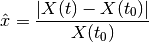
Before normalisation, the measurements that are out of the dynamic range [detection; saturation] are tagged to be ignored.
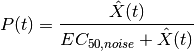
The fold change matrix is computed with a choice of algorithm. The following is the mode=”time” case (see normalise()):
Then, a penalty coefficient is computed as follows:
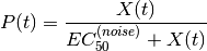
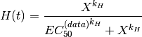
and the a new matrix is computed using a Hill transformation:
rescale negative values.
For each specy over all experiment and time, if a negative value is found and then the column is rescaled as follows:

where m_s and M_s are the minimum and maximum value over time and experiment for the given specy
.
- class XMIDASNormalise(data, mode='time', verbose=True, saturation=inf, detection=0.0, EC50noise=0.0, EC50data=0.5, HillCoeff=2.0, changeThreshold=0.0)[source]
This is a version of normalisation.
Note that it is 100 times slower than the version that uses numpy. However, it uses the XMIDAS datafrme as input and would be more convenient. Faster version could be implemented by providing a dataframe to numpy array.
Parameters: - EC50noise (float) – EC50noise no effect if set to 0 (defaults to 0)
- floatEC50Data – parameter for the scaling of the data between 0 and 1, default=0.5
- HillCoef (float) – Hill coefficient for the scaling of the data, default to 2
- EC50Noise – parameter for the computation of a penalty for data comparatively smaller than other time points or conditions. No effect if set to zero (default).
- detection (float) – minimum detection level of the instrument, -everything smaller will be treated as noise (NA), default to 0
- saturation (float) – saturation level of the instrument, everything over this will be treated as NA, default to Inf.
- changeThrehold (float) – threshold for relative change considered significant, default to 0
Once parameters are provided, you can still change them since there are all attributes. Thex next step is to normalise the data.
this can be done using one of :
- control_normalisation()[source]
In the control normalisation, the relative change is computed relative to the control experiment at the same time. The control being the experiment where all stimuli are zero but inhibitors re identical
Todo
check that a data set has these experiments.
Note
the time zero case is a special case. Indeed, even if provided, control is ignored. The t0 data is set to zero everywhere since only two measurements were made: with and without inhibitor(s) and these measurements have been copied across corresponding position; we assume that the inhibitors are already present at time 0 when we add the stimuli to find the right row to normalise.
Note
for now, the control is chosen as the experiment where all stimuli are zero.
changeTHresholdcan be a scalar or a time series (pandas) or a list
- time_normalisation()[source]
Class dedicated to the normalisation of MIDAS data
Before normalisation, the measurements that are out of the dynamic range [detection; saturation] are tagged to be ignored.
The fold change matrix is computed as follows:
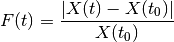
Then, a penalty coefficient is computed as follows:
where
 . A new matrix is computed using a Hill transformation:
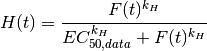
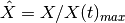
The data is first rescaled to take into account the noise and data:
Negative values are multiplied by -1 and values that are non-significant are set to zero.
Finally, rescale for min and max over each colum ignoring time t0 if and only if rescale_scaling is On.

where
 and
and  are the minimum and maximum value over time and
experiment for the given specy .
are the minimum and maximum value over time and
experiment for the given specy .Note
this normalisation works by computing a fold change relative to the same condition at time 0. If the value at time zero equals zero, , then the fold change calculation will fails. Note, however, that in X(t=0)=0 is not expected in many common biochemical techniques)
1.3. SIF
- class SIF(filename=None, format='cno', ignore_and=False, convert_ands=True)[source]
Manipulate network stored in SIF format.
The SIF format is used in Cytoscape and CellNOpt (www.cellnop.org). However, the format used in CellNOpt(R) restrict edges to be only 1 or -1. Besides, special nodes called AND nodes can be added using the “and” string followed by a unique identifier(integer) e.g., and22; seebelow for details.
See also
SIF section in the online documentation.
The SIF format is a tab-separated format. It encodes relations betwee nodes in a network. Each row contains a relation where the first column represents the input node, the second value is the type of relation. The following columns represents the output node(s). Here is a simple example:
A 1 B
B 1 C
A -1 B
but it can be factorised:
A 1 B C
B 1 C
In SIF, only OR reactions can be encoded. The following:
A 1 C
B 1 C
means A OR B gives C. AND reactions cannot be encoded therefore we have to code AND gates in a special way using a dedicated syntax. In order to encode the AND reaction the SIF reaction should be encoded as follows:
A 1 and1
B 1 and1
and1 1 C
An AND gate is made of the “and” string and a unique id concatenated as its end.
A SIF file can be read as follows:
s = SIF(filename)
Each line is transformed into reactions (A=B, !A=B). You can then add or remove reactions. If you save the file in a new SIF file, be aware than lines such as:
A 1 B C
are expanded as:
A 1 B
A 1 C
Aliases to the columns are stored in read-only attributes called nodes1, edges, nodes2. You can only add or remove reactions. Reactions are stored in reacID.
Todo
explain more precisely or simplify the 2 parameter ignore_and and convert_ands, which are different semantic ! one of r the ^ character, one for the and string.
Constructor
Parameters: - filename (str) – optional input SIF file.
- format (str) – “cno” or “generic” are accepted (default is cno). The cno format accepted only relation as “1” for activation, and “-1” for inhibitions. The “generic” format allows to have any relations. The “cno” format also interprets nodes that starts with “and” as logical AND gates.
- ignore_and (bool) – if you want to ignore the and nodes (see above), set to True.
- convert_ands (bool) – if AND nodes are found (from cellnopt syntax, eg a^b), converts them into a single reaction (default is True).
- add_reaction(reaction)[source]
Adds a reaction into the network.
Valid reactions are:
A=B
A+B=C
A^B=C
A&B=C
Where the LHS can use as many species as desired. The following reaction is valid:
A+B+C+D+E=F
Note however that OR gates (+ sign) are splitted so A+B=C is added as 2 different reactions:
A=C
B=C
- andNodes
Returns list of AND nodes
- data
Returns list of relations
- edges
returns list of edges found in the reactions
- export2SBMLQual(filename=None, modelName='CellNOpt_model')[source]
Exports SIF to SBMLqual format.
Parameters: - filename – save to the filename if provided
- modelName (str) – name of the model in SBML document
Returns: the SBML text
This is a level3, version1 exporter.
>>> s = SIF()
>>> s.add_reaction("A=B")
>>> res = s.export2SBMLQual("test.xml")
Warning
logical AND are not encoded yet. works only if no AND gates
Warning
experimental
- importSBMLQual(filename, clear=True)[source]
import SBMLQual XML file into a SIF instance
Parameters: - filename (str) – the filename of the SBMLQual
- clear (bool) – remove all existing nodes and edges
Warning
experimental
- namesSpecies
alias to specID
- nodes1
returns list of nodes in the left-hand sides of the reactions
- nodes2
returns list of nodes in the right-hand sides of the reactions
- plot()[source]
Plot the network
Note
this method uses cellnopt.core.cnograph so AND gates appear as small circles.
- reacID
- remove_reaction(reaction)
Remove a reaction from the reacID list
>>> c = Interactions()
>>> c.add_reaction("a=b")
>>> assert len(c.reacID) == 1
>>> c.remove_reaction("a=b")
>>> assert len(c.reacID) == 0
- remove_species(species_to_remove)
Removes species from the reacID list
Parameters: species_to_remove (str,list) – Note
If a reaction is “a+b=c” and you remove specy “a”, then the reaction is not enterely removed but replace by “b=c”
- save(filename, order='nodes1')[source]
Save the reactions (sorting with respect to order parameter)
Parameters: - filename (str) – where to save the nodes1 edges node2
- order (str) – can be nodes1, edges or nodes2
- search(specy, strict=False, verbose=True)
Prints and returns reactions that contain the specy name
Decomposes reactions into species first
Parameters: - specy (str) –
- strict (bool) – decompose reaction search for the provided specy name
Returns: a Interactions instance with relevant reactions
- sif2reaction()[source]
Returns a Reactions instance generated from the SIF file.
AND gates are interpreted. For instance the followinf SIF:
A 1 and1
B 1 and1
and1 1 C
give:
A^B=C
- specID
return species
- valid_symbols = ['+', '!', '&', '^']
2. Converters
2.1. SIF2ASP module
This module provides tools to convert a SIF file into a format appropriate to check sign consistency with ASP tools:
A 1 B
A -1 C
converted to
A -> B +
A -> C -
- class SIF2ASP(filename=None)[source]
Class to convert a SIF file into a ASP sign consistency format
>>> from cellnopt.core import SIF2ASP
>>> from cellnopt.data import cnodata
>>> filename = cnodata("PKN-ToyMMB.sif")
>>> s = SIF2ASP(filename)
>>> s.write2net("PKN-ToyMMB.net")
Constructor
Parameters: filename (str) – the SIF filename - signs
get the signs of the reactions
2.2. asp module
ASP related
- class NET(filename=None)[source]
Class to manipulate reactions in NET format.
The NET format
species1 -> species2 sign
where sign can be either the + or - character.
Examples are:
A -> B +
A -> B -
constructor
Parameters: filename (str) – optional filename containing NET reactions if provided, NET reactions are converted into reactions (see cellnopt.core.reactions.Reactions - net
- net2reaction(data)[source]
convert a NET string to a reaction
a NET string can be one of
A -> B +
C -> D -
where + indicates activation and - indicates inhibition
>>> assert net2reaction("A -> B +") == "A=B"
>>> assert net2reaction("A -> B -") == "!A=B"
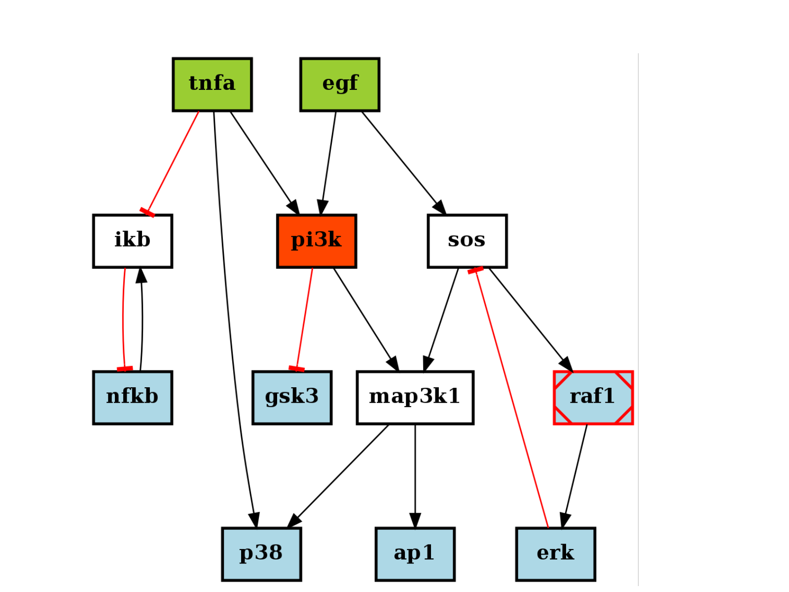
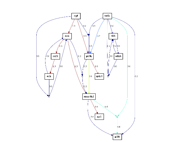
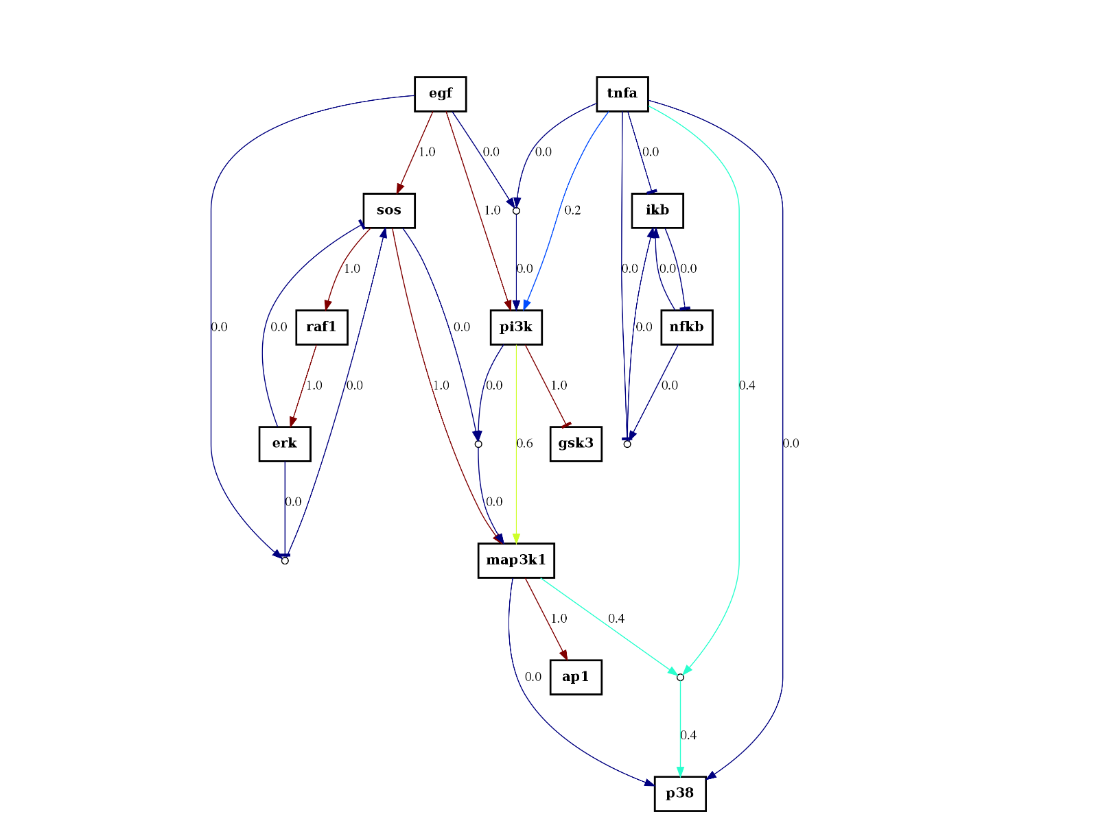
- class CASPOModels(filename)[source]
Class to read and plot models as exported by CASPO
>>> from cellnopt.core import *
>>> filename = get_share_file("caspo_models.csv")
>>> m = asp.CASPOModels(filename)
>>> m.plotdot(model_number=0)  # indices are m.df.index
>>> m.plotdot() # average model, whcih can be obtained with  m.get_average_model()
(Source code, png, hires.png, pdf)

Note
One difficulty is the way ANDs are coded in different software. In CASPO, the AND gate is coded as “A+B=C”. Note that internally we use ^ especially in CNOGraph. Then, an AND edge is splitted in sub edges. so, A+B=C is made of 3 edges A -> A+B=C , B -> A+B=C and A+B=C -> C. This explains the wierd code in plotdot().
2.3. ADJ2SIF module
- class ADJ2SIF(filenamePKN=None, filenameNames=None, delimiter=', ')[source]
Reads an adjacency matrix (and names) from CSV files
The instance can then be exported to SIF or used as input for the cellnopt.core.cnograph.CNOGraph structure.
>>> from cellnopt.core import *
>>> f1 = get_share_file("adjacency_matrix.csv")
>>> f2 = get_share_file("adjacency_names.csv")
>>> s = ADJ2SIF(f1, f2)
>>> sif = s.export2sif()
>>> c = CNOGraph(s.G)

Where the adjacency matrix looks like::

    0,1,0
    1,0,0
    0,0,1

and names is a 1-column file::

    A
    B
    C

The exported SIF file would look like::

    A 1 B
    A 1 C
Warning
The adjacency matrix contains only ones (no -1) so future version may need to add that information using incidence matrix for instance
Todo
could use pandas to keep names and data altogether.
Constructor
Parameters: - filenamePKN (str) – adjacency matrix made of 0’s and 1’s.
- filenameNames (str) – names of the columns/rows of the adjacency matrix
- delimiter (str) – commas by default
0,1,0
1,0,0
0,0,1
names:
A
B
C
The 2 files above correspond to this SIF file:
A 1 B
A 1 C
- G
The graph created from
- export2sif(filename=None)[source]
Exports input data files into a SIF instance and save it
Parameters: filename (str) – set this parameter if you want to save the SIF into a file Returns: a SIF instance
- load_adjacency(filename=None)[source]
Reads the adjacency matrix filename
if no filename is provided, tries to load from the attribute filename.
- names
Names of the nodes read from the the provided filename
2.4. SOP2SIF module
- class SOP2SIF(filename)[source]
Converts a file from SOP to SIF format
SOP stands for sum of products, it is a list of relations of the form:
!A+B=C
For now, this function has been tested and used on the copy/paste of a PDF document into a file. Be careful because the interpretation of the characters may differ from one distribution to the other. The original data contains
- a special character for NOT, which is interpreted as x2xac (a L turned by 90 degrees clockwise)
- an inversed ^ character for OR, which is interpreted as ” _ “
- a ^ character for AND, which is correctly interpreted.
- a -> character for “gives”, which is transformed into ! character.
On other systems, it may be interpreted differently, so we provide a mapping attribute mapping to perform the translation, which can be changed to your needs.
The data looks like:
1 !A + B = C 1 [references]
2 !A + B = E 2 [references]
3 !A + B = D 1 [references]
...
N !A + B = D 2 [references]
The SOP2SIF class gets rid of the last column, the [references] and the column before it (made of 1 and 2). Then, we convert the reaction strings into the same format as in CellNOpt that is:
- A = C means A GIVES C
- A + B = C means A gives C OR B gives C
- !A means NOT A
>>> s2s = SOP2SIF("data.sop")
>>> s = s2s.sop2sif()
>>> s2s.writeSIF("data.sif")
- export2sif(filename, include_and_gates=True)[source]
Save the reactions in a file using SIF format
The data read from the SOP file is transformed into a SIF class before hand.
Parameters: include_and_gates (bool) – if set to False, all reactions with AND gates removed
- mapping = None
The dictionary to map SOP special characters e.g if you code NOT with ! character, just fill this dictionary accordingly
- sop2sif(include_and_gates=True)[source]
Converts the SOP data into a SIF class
Parameters: include_and_gates (bool) – if set to False, all reactions with AND gates are removed. Returns: an instance of cellnopt.core.sif.SIF
2.5. EDA module
- class EDA(filename, threshold=0, verbose=False)[source]
Reads networks in EDA format
EDA format is similar to SIF but provides a weight on each edge.
So, it looks like:
A (1) B = .5
B (1) C =  1
A (1) C = .1
Parameters: - filename (str) –
- threshold (float) – should be between 0 and 1 but not compulsary
- verbose (bool) –
- export2sif(threshold=None)[source]
Exports EDA data into SIF file
Parameters: threshold (float) – since EDA format provides a weight on each edge, it can be used as a threshold to consider the relation or not. By default, the threshold is set to 0, which means all edges should be exported in the output SIF format (assuming weights are positive). You ca n either set the threshold attribute to a different value or provide this threshold parameter to override the default threshold. >>> from cellnopt.core import eda >>>from cellnopt.core import get_share_file as gsf >>> e = EDA((gsf("simple.eda)) >>> s1 = e.export2sif() # default threshold 0 >>> len(s1) 3 >>> s1 = e.export2sif(0.6) # one edge with weight=0.5 is ignored >>> len(s1) 2
3. Others
3.1. Interaction class
This module contains a base class to manipulate reactions
Todo
merge Interactions and Reactions class together
- class Interactions(format='cno', strict_rules=True)[source]
Interactions is a Base class to manipulate reactions (e.g., A=B)
You can create list of reactions using the =, !, + and ^ characters with the following meaning:
   >>> from cellnopt.core import *
   >>> c = Interactions()
   >>> c.add_reaction("A+B=C") # a OR reaction
   >>> c.add_reaction("A^B=C") # an AND reaction
   >>> c.add_reaction("A&B=C") # an AND reaction
   >>> c.add_reaction("C=D")   # an activation
   >>> c.add_reaction("!D=E")  # a NOT reaction

#. The **!** sign indicates a NOT logic.
#. The **+** sign indicates a OR.
#. The **=** sign indicates a relation.
#. The **^** or **&** signs indicate an AND ut **&** are replaced by **^**.
Warning
meaning of + sign is OR so A+B=C is same as 2 reactions: A=C, B=C
Now, we can get the species:
>>> c.specID
['A', 'B', 'C', 'D', 'E']
Remove one:
>>> c.remove_species("A")
>>> c.reacID
["B=C", "C=D", "!D=E"]
See also
- add_reaction(reaction)[source]
Adds a reaction in the list of reactions
In logical formalism, the inverted hat stand for OR but there is no such key on standard keyboard so we use the + sign instead. The AND is defined with either the ^ or & sign. Finally the NOT is defined by the ! sign. Valid reactions are therefore:
a=b
a+c=d
a&b=e
a^b=e  # same as above
!a=e
Example:
>>> c = Interactions()
>>> c.add_reaction("a=b")
>>> assert len(c.reacID) == 1
- namesSpecies
alias to specID
- reacID
- remove_reaction(reaction)[source]
Remove a reaction from the reacID list
>>> c = Interactions()
>>> c.add_reaction("a=b")
>>> assert len(c.reacID) == 1
>>> c.remove_reaction("a=b")
>>> assert len(c.reacID) == 0
- remove_species(species_to_remove)[source]
Removes species from the reacID list
Parameters: species_to_remove (str,list) – Note
If a reaction is “a+b=c” and you remove specy “a”, then the reaction is not enterely removed but replace by “b=c”
- search(specy, strict=False, verbose=True)[source]
Prints and returns reactions that contain the specy name
Decomposes reactions into species first
Parameters: - specy (str) –
- strict (bool) – decompose reaction search for the provided specy name
Returns: a Interactions instance with relevant reactions
- specID
return species
- valid_symbols = ['+', '!', '&', '^']
- class Reaction(reaction=None, strict_rules=True)[source]
A Reaction class
A Reaction can encode logical AND and OR as well as NOT:
>>> from cellnopt.core import Reaction
>>> r = Reaction("A+B=C") # a OR reaction
>>> r = Reaction("A^B=C") # an AND reaction
>>> r = Reaction("A&B=C") # an AND reaction
>>> r = Reaction("C=D")   # an activation
>>> r = Reaction("!D=E")  # a NOT reaction

    r.name
    r.rename_species(old, new)
    r._valid_reaction("a=b")
Parameters: - reaction (str) –
- strict_rules (bool) – if True, reactions cannot start with =, ^ or ^ signs.
- name
- rename_species(old, new)[source]
difficulties: (1) if a species is called BAC, replace A by D must not touch BAC names (2) delimiters such as !, +, ^ should be taken into account
- valid_symbols = ['+', '!', '&', '^']
3.2. kinexus
Module dedicated to convertion of kinexus data into MIDAS
- class Kinexus(filename=None, sheet=None, header_uniprot='Uniprot_Link', header_protein_name='Target_Protein_Name', sep=':', **kargs)[source]
Class dedicated to kinexus data
The Kinexus data are provided as Excel documents with several sheets. The main sheet called “kinetic” contains all the relevant data. It can be a pure excel document or a CSV file with separator as : character.
The following columns are looked for:
- Target Protein Name
- Uniprot Link
- Globally Normalized TXX where XX is a time
See Constructor for more information about the CSV format.
>>> k = Kinexus("kinetic.csv")
>>> k.data
>>> k.select_globally_normalised()
>>> k.export2midas()
Constructor
Parameters: filename (str) – the file is a CSV file that was exported from an excel document (sheet called kinetic). Make sure the header is on 1 single line. Strings are bracketed with double quotes. CSV file means comma separated but we used ”:” character as a delimiter since spaces and commas may be used within cells. In LibreOffice, “save as” your excel and set the field delimiter to ”:” character. Set Text delimiter no nothing. If you do not provide a filename, you cannot export to midas but you can still play with some methods such as get_name_from_uniprot().
This class will try to identify the meaning of the columns. We want to retrieve the data at different time points given the target protein name or antibody names. Kinexus daa may be diverse so there is no guarantee that this class will work for a variety of different input format.
The data at different time points are extracted from the column that are tagged “Globally Normalized TX” where X is the time tag (e.g., 0, 1, 5) All columns starting with “Globally” are extracted. The different times are stored. (see select_globally_normalised().
get_name_from_uniprot() retrieve the exact UniProt name given a uniprot accession number, which is more meaningful.
Several rows may target the same protein with the same uniprot ID. So, we need to differentiate them in the data. This is done by appending the phosphosite to the target protein name.
- columns
- data
- export2midas(filename='MD-kinexus.csv', mode='globally_normalised', uniprot=True)[source]
Converts the Kinexus data into a MIDAS file.
Parameters: - filename (str) – the output name for the MIDAS file
- mode (str) – There are different post processed data in the Kinexus data so we used a mode to refine what user can export in the MIDAS file. Right now only one mode is allowed that is “globally_normalised”. See select_globally_normalised() method for details.
- uniprot (bool) – specy names in the MIDAS file will be the UniProt Entry Name. Otherwise, the hand-written “Target Protein Names”
Note
row with no uniprot (ie. set to NA) are ignored
- get_name_from_uniprot(Id, taxon=9606)[source]
Get unique Entry Name (without specy) from a unique uniprot ID
Parameters: - Id (str) – UniProt ID (e.g., P43403)
- taxon (str) – the specy taxon. 9606 correspond to HUMAN
Returns: the name without taxon (e.g., ZAP70)
>>> k = Kinexus()
>>> k.get_name_from_uniprot("P43403")
'ZAP70'
Todo
a global mapping that is much faster using : u.mapping(“ACC”, “ID”, ” ”.join(k.df.Uniprot_Link))
- header_uniprot = None
can be changed to fit your data
- index
- read_csv(filename, **kargs)
- read_excel(filename, sheet, **kargs)
- select_globally_normalised()[source]
Returns a subset of the entire data set
The selection is the protein name, followed by the data at different time point labelled “Globally Normalised” and finally the uniprot ID. The number of time points and their values can be retrieved from _get_times() method
protein names are obtained from the uniprot ID given in the kinexus data.
Returns: list of tuples. Each tuple contain the data as exaplained above (protein name, data, uniprot ID)
3.3. Reactions module
Module dedicated to the CNA reactions data structure
| Status: | for production but not all features implemented. |
|---|
- class Reactions(filename=None, type=2, verbose=False)[source]
Reads a reaction file (CNA format)
This class has the Interaction class as a Base class. It is used to read reactions files from the CNA format, which is a CSV-like format where each line looks like:
mek=erk 1 mek = 1 erk | # 0 1 0 436 825 1 1 0.01
The pipe decompose the strings into a LHS and RHS.
The LHS is made of a unique identifier without blanks (mek=erk). The remaining part is the reaction equation. The equal sign “=” denotes the reaction arrow. Identifiers, coefficients and equal sign must be separated by at least one blank. The ! sign to indicate not. The + sign indicates an OR relation.
Warning
The + sign indicates an OR as it should be. However, keep in mind that in CellNOptR code, the + sign indicates an AND gate. In this package we always use + for an OR and ^ or & for an AND gate.
Warning
in the CNA case, some reactions have no LHS or RHS. Such reactions are valid in CNA but may cause issue if converted to SIF
Note
there don’t seem to be any AND in CNA reactions.
The RHS is made of
a default value: # or a value.
- a set of 3 flags representing the time scale
- flag 1: whether this interaction is to be excluded in logical computations
- flag 2: whether the logical interaction is treated with incomplete truth table
- flag 3: whether the interaction is monotone
reacBoxes (columns 5,6,7,8)
monotony (col 9)
In this class, only the LHS are used for now, however, the RHS values are stored in different attributes.
>>> from cellnopt.core import *
>>> a = Reactions(get_share_file('reactions'))
>>> reacs = a.reacID
>>> # a.writeSIF("test.sif")
Constructor
Parameters: - filename (str) – an optional filename containing reactions in CNA format. If not provided, the Reactions object is empty but you can add reactions using add_reaction(). However, attributes such as reacBoxes will not be populated.
- type (integer) – only type 2 for now.
- verbose (bool) – False by default
Todo
type1 will be implemented on request.
- add_reaction(reaction)
Adds a reaction in the list of reactions
In logical formalism, the inverted hat stand for OR but there is no such key on standard keyboard so we use the + sign instead. The AND is defined with either the ^ or & sign. Finally the NOT is defined by the ! sign. Valid reactions are therefore:
a=b
a+c=d
a&b=e
a^b=e  # same as above
!a=e
Example:
>>> c = Interactions()
>>> c.add_reaction("a=b")
>>> assert len(c.reacID) == 1
- excludeInLogical = None
populated when reading CNA reactions file
- incTruthTable = None
populated when reading CNA reactions file
- monotony = None
populated when reading CNA reactions file
- namesSpecies
alias to specID
- reacBoxes = None
populated when reading CNA reactions file
- reacID
- reacText = None
populated when reading CNA reactions file
- remove_reaction(reaction)
Remove a reaction from the reacID list
>>> c = Interactions()
>>> c.add_reaction("a=b")
>>> assert len(c.reacID) == 1
>>> c.remove_reaction("a=b")
>>> assert len(c.reacID) == 0
- remove_species(species_to_remove)
Removes species from the reacID list
Parameters: species_to_remove (str,list) – Note
If a reaction is “a+b=c” and you remove specy “a”, then the reaction is not enterely removed but replace by “b=c”
- search(specy, strict=False, verbose=True)
Prints and returns reactions that contain the specy name
Decomposes reactions into species first
Parameters: - specy (str) –
- strict (bool) – decompose reaction search for the provided specy name
Returns: a Interactions instance with relevant reactions
- specID
return species
- timeScale = None
populated when reading CNA reactions file
- valid_symbols = ['+', '!', '&', '^']
- writeSIF(filename=None)[source]
Export the reactions to SIF format
from cellnopt.core import *
r = Reactions()
r.add_reaction("a=b")
r.add_reaction("a+c=e")
r.writeSIF("test.sif")
Again, be aware that “+” sign in Reaction means “OR”. Looking into the save file, we have the a+c=e reactions (a=e OR c=e) expanded into 2 reactions (a 1 e) and (c 1 e) as expected:
a   1   b
a   1   e
c   1   e
3.4. Metabolites module
Module dedicates to the metabolites CNA format
| Status: | mature but not all features implemented. |
|---|
Based on load_substances_inter matlab version provided by Steffen, Klamt, MPI “Dynamik komplexer technischer Systeme” Magdeburg
- class Metabolites(filename, verbose=True)[source]
Read metabolites file and convert to a Metabolites data structure.
Metabolites format is a CSV format that looks like:
abl         abl         NaN     0   188  380    1    1
akap79      akap79      NaN     0   989  442    1    1
Columns are
identifier of this substance in CNA (e.g.: G6P) without blanks stored in specID
- the full name of the metabolite (e.g.: glucose-6-phosphate; no blanks
allowed!) stored in specLongNames
could be # or a value stored in specDefault
a value 0/1 (ignored right now)
4 following columns must be numerical values stored in specBoxes
Todo
specify precicely the content of the columns
>>> from cellnopt.core import Metabolites
>>> m = Metabolites("metabolites")
>>> m.specID
Constructor
Parameters: - filename (str) – input filename containing the metabolites data
- verbose (bool) – (True by default)
- specBoxes = None
attribute to store specBoxes
- specDefault = None
attribute to store spec default
- specID = None
attribute to store the specID
- specLongNames = None
attribute to store the specLongNames
- specNotes = None
attributes to store specNotes