2. User Guide
Contents
2.1. The different formats
There are quite a few formats out there and cellnopt.core provides some converters.
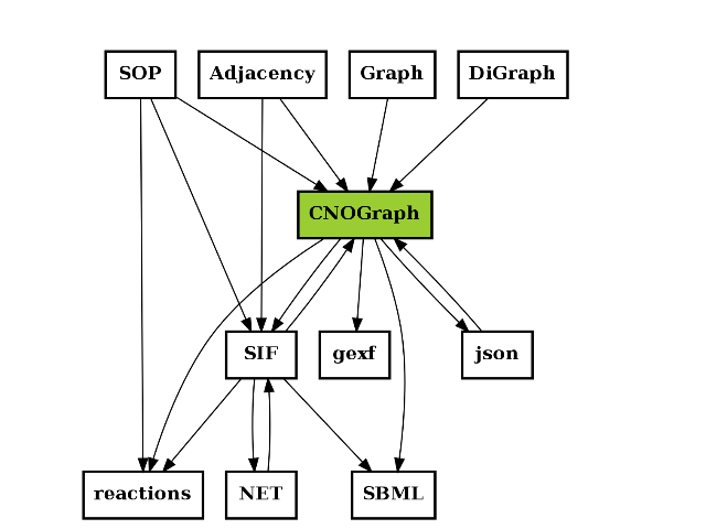
The following image is not stricly speaking complete but give an idea of what formats are used and how they are linked together.
A relation A to B may mean (i) A can be exported to B or A can be an input to B (or loaded).
For instance CNOGraph can take as input a SIF instance or a filename that links to a SIF file. Conversely it can export a SIF into a file. CNOGraph can be saved into a json that can be then loaded (loadjson).
See also
from cellnopt.core import *
c = CNOGraph()
c.add_reaction('SOP=reactions')
c.add_reaction('SOP=CNOGraph')
c.add_reaction('SOP=SIF')
c.add_reaction('SIF=reactions')
c.add_reaction('SIF=CNOGraph')
c.add_reaction('Adjacency=SIF')
c.add_reaction('Adjacency=CNOGraph')
c.add_reaction('Graph=CNOGraph')
c.add_reaction('DiGraph=CNOGraph')
c.add_reaction('SIF=CNOGraph')
c.add_reaction('SIF=SBML')
c.add_reaction('CNOGraph=reactions')
c.add_reaction('CNOGraph=json')
c.add_reaction('CNOGraph=SBML')
c.add_reaction('CNOGraph=SIF')
c.add_reaction('CNOGraph=gexf')
c.add_reaction("json=CNOGraph")
c.add_reaction("NET=SIF")
c.add_reaction("SIF=NET")
c._stimuli = ["CNOGraph"]
c.plotdot()
(Source code, png, hires.png, pdf)

2.1.1. SIF
The SIF format is a cytoscape compatible format, which is just a space or tab separated value format. The advantage is its simplicity. Here is an example:
specy1 1 specy2
specy1 1 specy3
with the disadvantage that this format does not include any layout information and comments cannot be added.
Each line in a SIF file represents an interaction between a source (left) and one or more target nodes (right):
nodeA relationship nodeB
nodeC relationship nodeA
nodeD relationship nodeE nodeF nodeB
The SIF format used in CellNOpt is actually a subset of the official SIF format:
Generally there is only one target
The relationship can be only the number 1 or -1 (for inhibitor)
Duplicated entries are not ignored but only the latest is taken into account
OR relations are implicit: a relation “A 1 C” and a relation “B 1 C” should be understood as A OR B gives C
special word “and” is used to code an AND relationship. An AND gate requires 3 relations:
A 1 and1
B 1 and1
and1 1 C
Delimiters can be spaces or tabs (mixed).
With cellnopt.core, you can create a SIF instance from scratch and populate it as follows:
>>> s1 = SIF()
>>> s1.add_reaction("A=C")
>>> s1.add_reaction("B=C")

>>> #or simply:
>>> s2 = SIF()
>>> s2.add_reaction("A+B=C")
Some operators are available:
>>> s2 == s
True
There is no plotting functions associated with the SIF class but you can easily create a CNOGrapg instance and plot the model:
c = CNOGraph(s)
c.plotdot()
2.1.2. MIDAS
The MIDAS (Minimum Information for Data Analysis in Systems Biology) format is used in CellNOpt software. For more details, please see [DataRail1] and [DataRail2].
An example of a MIDAS file looks like:
TR:mock:CellLine, TR:EGF, TR:TNFa, TR:PI3Ki, DA:Akt, DA:Hsp27, DV:Akt, DV:Hsp27
1,                1,      0,       0,        0,      0,        0,      0
1,                0,      1,       0,        0,      0,        0,      0
1,                1,      0,       0,        10,     10,       0.82,   0.7
1,                0,      1,       0,        10,     10,       0.91,   0.7
2.1.2.1. Format
MIDAS files are CSV files (comma separated). The content is defined in the first line of the file that constitutes the header (only 1 line). In the header, colums can take two forms:
XX:userword
XX:userword:category
where XX is a 2-letter word prefix that describes the column content (see table below for valid word), userword is a word provided by the user that could be the protein name. Category is a keyword that is optional except for the cell lines names. Category could be one of CellLine, Stimuli or Inhibitors. In practice Stimuli is never used. Inhibitors could be used to alleviate ambiguity coming from the MIDAS format when defining inhibitors (see below). Some MIDAS file encode other categories (e.g. cyto, NOLIG) but there are ignored in CellNOptR and cellnopt.core.
MIDAS files include the concept of cues, signals, and responses (Gaudet et al., 2005):
- cues are biological perturbations to a system (such as the addition of extracellular ligands)
- signals represent the activities of proteins or other biomolecules involved in transducing biological information (activation of an intracellular kinase, for example),
- responses also called readouts represent phenotypic changes such as proliferation, cell death or cytokine release.
In MIDAS, cues can be stimuli or inhibitors. Signals and responses are measurements made on species (the specy usage does not correspond to human or mouse but protein/kinases,phenotype...)
| Code | Description | handled in CellNOptR |
|---|---|---|
| ID | identifiers | ignored but stored |
| TR | treatment | yes |
| DA | Data aquistion | yes |
| DV | Data value | yes |
| other | ignored but stored |
Example:
| TR:mock:CellLine | TR:EGF | TR:TNFa | TR:PI3Ki | DA:Akt | DA:Hsp27 | DV:Akt | DV:Hsp27 |
|---|---|---|---|---|---|---|---|
| 1 | 1 | 0 | 0 | 0 | 0 | 0 | 0 |
| 1 | 0 | 1 | 0 | 0 | 0 | 0 | 0 |
| 1 | 1 | 0 | 0 | 10 | 10 | 1 | 0.2 |
| 1 | 0 | 1 | 0 | 10 | 10 | 1 | 0.5 |
Each value is separated by a comma and you could have space, tabs between commas. So, the final format could be as follows:
TR:mock:CellLine, TR:EGF, TR:TNFa, TR:PI3Ki, DA:Akt, DA:Hsp27, DV:Akt,DV:Hsp27
1,1,0,0, 0,0,   0,0
1,0,1,0, 0,0,   0,0
1,1,0,0, 10,10, 0.82,0.7
1,0,1,0, 10,10, 0.91,0.7
More details about the header
- The first row is the header describing the content of each colum.
- commas separate all fields.
- Valid code (e.g., TR) must be followed by a column (e.g., TR: or DA:).
- additional category can be added: TR:EGF:Stimuli
- Special fields such as NOCYTO and NOINHIB are ignored.
- The number of DA and DV must be equal except if you use the special name DA:ALL (see later).
- Inhibitors are coded by adding the letter i after the name (e.g., TR:PI3Ki) If this lead to ambiguity (i.e., a specy ends with i) then use the Inhibitor or Stimuli category (e.g., TR:PI3Ki:Stimuli
The data above is made of rows that length is as long as the header. Fields may may be empty, which is not the case here. If so, software should replace the value by (e.g., NA in R language) and cope with it.
Each row represents a given treatment at a given time. Times are coded with the DA code. Values are coded within the DV columns. In the 2 first rows the time is 0. The next two other rows are coded for the time 10. The treatements (3 first colums) are found at the different time.
In MIDAS file, data should be ordered by time although some software may deal with it.
2.1.2.2. Filename issue
From [DataRail1]:
MIDAS file has a unique identifier (UID) composed of the following fields:
(i) a two-letter data/file-type code (e.g., PDfor Primary Data, MD for
multiplex data), (ii) a three-letter creator code (typically initials),
(iii) an identification number of arbitrary length that is unique across
the entire system, and (iv) a free-text suffix that serves as a mnemonic
to improve human readability. For example, the primary data discussed in
the text might be tagged MD-LGA-11111-CytoInh17phFI-BLK
In practice, only a few files are coded that way. One reason is that the UID tag is hardly used. Another inconsistency is that dashes are not used or replaced by _. Besides, many files contain the word Data. Finally, the name tag (e.g. LGA above) is not good practice because public file should give the feeling they belong to everybody. However, one consistency is the extension being .csv.
2.1.2.3. Proposal for filename convention
- do not use the DATA/Data word. Instead start all files with MD- and use the extension .csv
- separate the names that describe your data with dashes.
- Underscore could be use internally to refine a name
- MD must be capitalised, other names can use any convention but we recomment polish convention (e.g., capitalize words)
MD-Tag1-Tag2.csv
MD indicates that this is a MIDAS file so no need to set Data in the filename anymore. Tag1 is a general description tag (containing _ possibly) and Tag2 is a variant of Tag1. For instance, Tag1 could be Toy and Tag2 a name to differentiate different Toy data sets.
Correct:
MD-Toy.csv
MD-Toy-variant1.csv
MD-LiverDream.csv
MD-LiverDREAM.csv
2.1.3. CNA Reactions
CNA reactions is a CSV-like format. Lines looks like:
mek=erk 1 mek = 1 erk | # 0 1 0 436 825 1 1 0.01
The first column contains the reactions (mek=erk). Following columns until the “|” sign decompose the reactions using a space to separate each component of the reaction. After the “|” sign, there are 9 extra columns.
You can read CNA reactions. You can then convert them into SIF and CNOGraph before plotting the graph:
from cellnopt.core import *
a = Reactions(get_share_file('reactions'))
s = SIF()
for x in a.reacID: s.add_reaction(x)
c = CNOGraph(s)
c.plotdot()
Note
future version may allow to directly read the CNA file from the CNOGraph structure itself.
See cellnopt.core.reactions.Reactions class for more details.
2.1.4. CNA Metabolites
Metabolites format is a CSV format that looks like:
abl         abl         NaN     0   188  380    1    1
akap79      akap79      NaN     0   989  442    1    1
You can read this file using cellnopt.core.metabolites.Metabolites class:
>>> from cellnopt.core import Metabolites, get_share_file
>>> filename = get_share_file("metabolites")
>>> m = Metabolites(filename)

Reading Species ...
Found an empty line. Skipped
Found 94 species
No valid notes were found. Skipping.
2.1.5. SOP
There is a function that converts SOP data file into SIF format in cellnopt.core.sop2sif.SOP2SIF
2.1.6. Kinexus
Kinexus data are in Excel format. There is no facility to read the Excel documentation directly and different format may be used. However, we can export the excel sheet into a CSV file that can be read by the cellnopt.core.kinexus.Kinexus class.
2.2. The CNOGraph data structure and plotting
The quick start already mentionned this data structure. Here is another example on how to play with the plotdot() plotting function. It relies on graphviz that must be installed but is quite convenient. Here is an example:
from cellnopt.core import *
c = cnograph.CNOGraph(get_share_file("PKN-Test.sif"), get_share_file("MD-Test.csv"))
import networkx as nx

# show a PNG image using matplotlib
c.plotdot()
(Source code, png, hires.png, pdf)
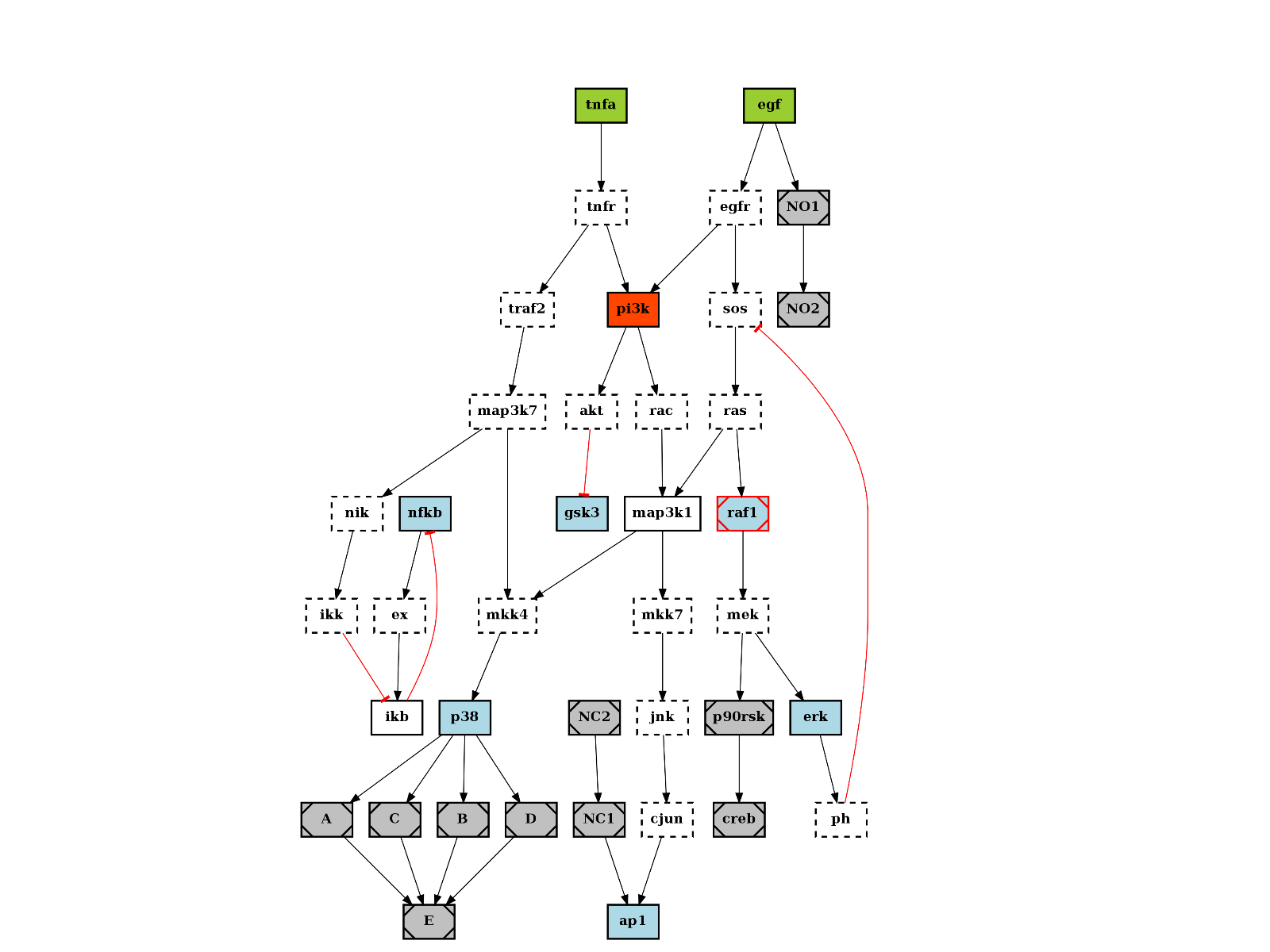
The plotdot function creates a dot file that is then shown within matplotlib. The node and edge attributes are set to default values using the MIDAS file provided (e.g., stimuli are green boxes).
Additional attributes can be set if there are valid graphviz keywords. For instance, we can add a URL attribute that could be used when creating a SVG file:
c.node["tnfa"]["URL"] = "http://www.uniprot.org/uniprot/P01375"
similarly, graphviz option for the graph such as the resoultion (dpi), background color (bgcolor) can be set:
c.graph['graph'] = {"dpi":100,'splines':True, 'bgcolor':'red'}
nx.write_dot(c, "test.dot")
Play around with graphviz to add visible clusters:
import networkx as nx
G = nx.to_agraph(c)
G.add_subgraph(["A", "B", "C", "D"], name="cluster_1", label="test", fillcolor="#11ff11", color="black", style="filled")
G.write("test.dot")