1. Quick Start

1.1. The CNOGraph data structure

The CNOGraph data structure is a DiGraph data structure. The topology can be built in many different ways given various inputs (SIF, SBMLqual, a DiGraph, etc). A second optional parameter is a MIDAS file that contain measurements on nodes, which may be use to color nodes according to their function (e.g., ligands, readouts, ...)

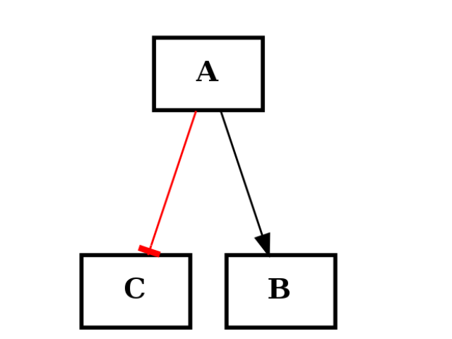
You can also start from scratch with an empty graph. However, there is a restriction on the type of edges that can be only of two types: “+” for activation and “-” for inhibition. The following example shows how to create a simple graph made of 3 nodes and 2 edges: one activation (black) and one inhibition (red):

from cellnopt.core import *
c1 = CNOGraph()
c1.add_edge("A","B", link="+")
c1.add_edge("A","C", link="-")
c1.plotdot()

(Source code, png, hires.png, pdf)

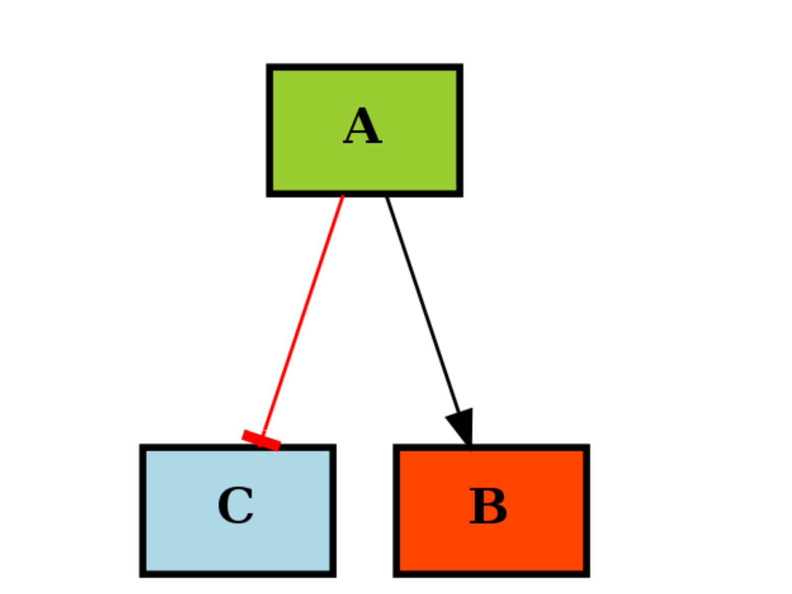
If you use a MIDAS file during the instanciation, the CNOGraph will color the nodes that are found in the MIDAS file. Stimuli (ligand) are colored in green, inhibitors in red and readout (signal) in blue. If you did not provide a MIDAS file, you can still specificy the list manually like in the following example:

from cellnopt.core import *
c1 = CNOGraph()
c1.add_edge("A","B", link="+")
c1.add_edge("A","C", link="-")
c1._stimuli = ["A"]
c1._inhibitors = ["B"]
c1._signals = ["C"]
c1.plotdot()

(Source code, png, hires.png, pdf)

There are many operators available and readers can refer to cellnopt.core.cnograph.CNOGraph for more examples.

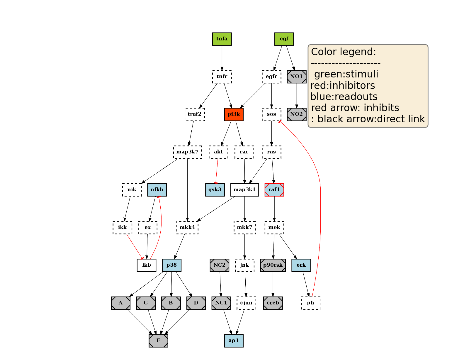
1.1.1. CNOGraph as a data structure to manipulate SIF/MIDAS file

The common data structure CNOGraph can also take as input a SIF instance and a MIDAS instance (or filenames). The latter is optional.

c = CNOGraph(s, m)

This data structure has many methods inherited from networkx.DiGraph class and many algorithms can be applied. The input SIF file is used to build the topology of the graph. The input MIDAS file if provided is used to set the color of the nodes and edges when calling plotting functions. Besides, with the information contained in the MIDAS file, functions similar to those in CellNOptR can be applied (pre processing functions to add AND gates, compress nodes that are not measured; see User Guide for details).

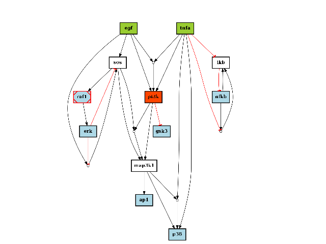
As an example, you can plot the graph using plotdot():

from cellnopt.core import *
s = SIF(get_share_file("PKN-Test.sif"))
m = XMIDAS(get_share_file("MD-Test.csv"))
c = CNOGraph(s, m)
c.plotdot(legend=True)

(Source code, png, hires.png, pdf)

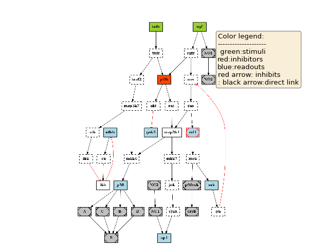
The CNOGraph structure provides methods to perform processing dedicated to CellNOpt analysis. This processing are made of three steps:

1. removal of non observable and non controlable
2. compress nodes that are not measured, not stimuli, not inhibited.
3. add AND gates

See cellnopt.core.cnograph.CNOGraph() class for details.

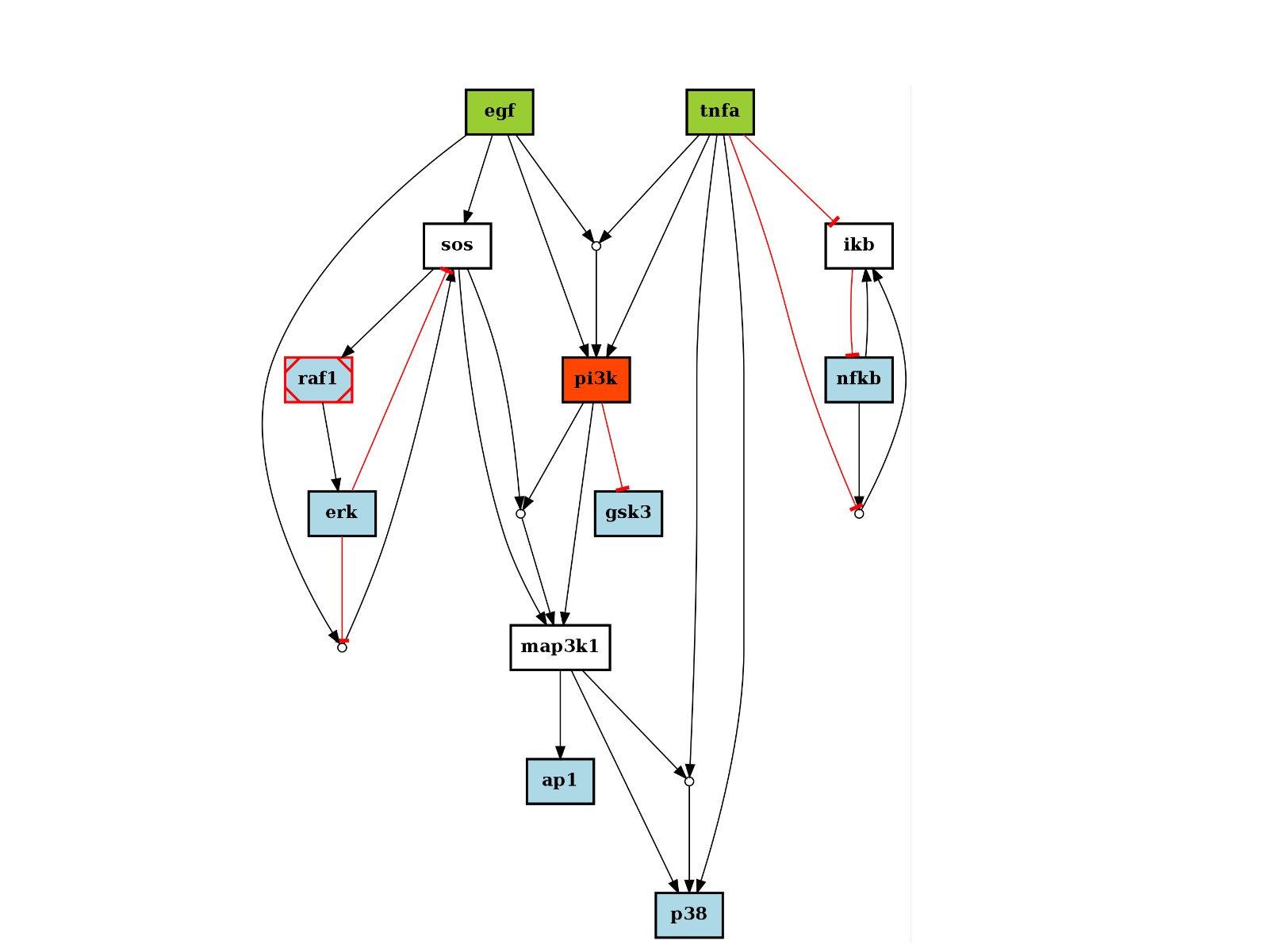
Let us apply these 3 steps and plot the graph again:

from cellnopt.core import *
s = SIF(get_share_file("PKN-Test.sif"))
m = XMIDAS(get_share_file("MD-Test.csv"))
c = CNOGraph(s, m)
c.preprocessing()
c.plotdot()

(Source code, png, hires.png, pdf)

1.2. Read data files in SIF and MIDAS formats

To begin, the easiest is to import the entire package to get access to all classes and functions:

>>> from cellnopt.core import *

In order to use some of the functionalities, we need some sample data sets. We will play with a protein-protein interactions network coded in (SIF format) and a data set that stores signalling data stored in MIDAS format. The package cellnopt.core provides samples to play with, which can be obtained using the cnodata() function (part of another package called cellnopt.data.tools.cnodata() but linked within cellnopt.core for convenience):

>>> sifFilename = cnodata("PKN-ToyPB.sif")
>>> midasFilename = cnodata("MD-ToyPB.csv")

Alternatively, you can also use get_share_file() to obtain test samples provided within cellnopt.core package itself:

>>> from cellnopt.core import get_share_file
>>> get_share_file("PKN-Test.sif")

Once you’ve chosen a filename, you can create a SIF instance as follows:

>>> s = SIF(sifFilename)

and a XMIDAS instance as follows:

>>> m = XMIDAS(midasFilename)

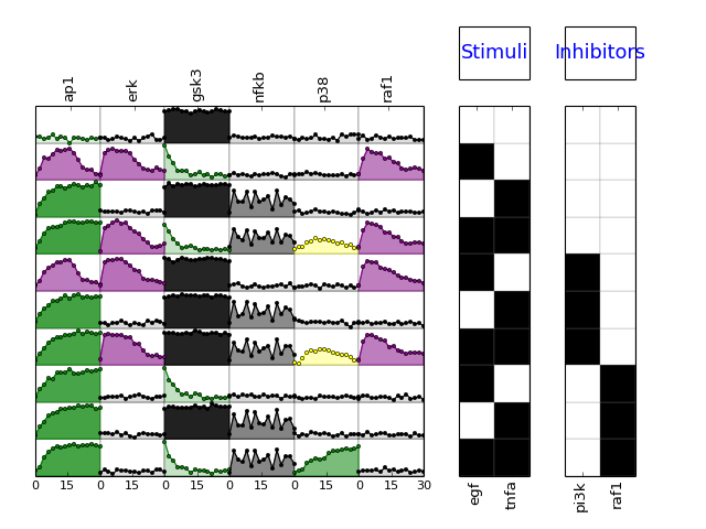
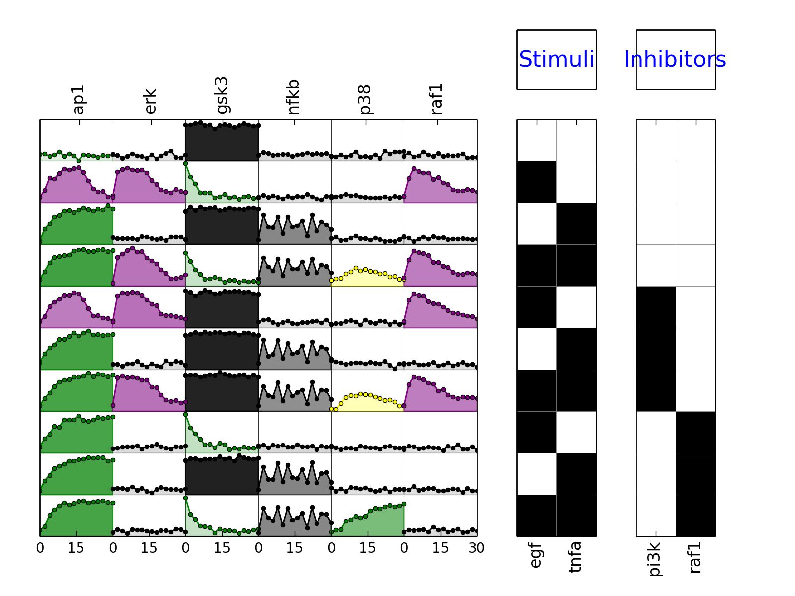
These two objects m and s have many methods and users should refer to the reference guide for an exhaustive documentation. As an example, we can plot the data contained in the MIDAS file:

>>> m.plotMSEs()
>>> m.plotExp()

(Source code, png, hires.png, pdf)