Back to Guide
Space tutorial
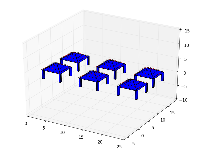
Example of a Space with six individual Places.
-
class
pyny3d.geoms.Space(places=[], **kwargs)[source] the highest level geometry class. It Aggregates
pyny.Placesto group computations. It can be initialized empty.- The lower level instances will be stored in:
- Space.places
Parameters: places (list of pyny.Place) – Places or empty list.Returns: None Instances of this class work as iterable object. When indexed, returns the
pyny.Placeswhich conform it.Note
This class is implemented to be used dynamically. Once created, it is possible to add elements, with
.add_places,.add_spacesamong others, without replace it.Warning
Although it is a dynamic class, it is recommended to use the methods to manipulate it. Editing the internal attributes or methods directly can result in a bad behavior.
Non-trivial methods
As always, you can also use the Space documentation for method-by-method description, specially for the trivial methods we are going to skip in this section.
Trivial methods:
method description .add_places() Add new places to the space .add_space() Merge other spaces with this one .add_set_of_points() Add a set of points .clear_set_of_points() Remove the points in this place .explode() Collect all the polygons, holes and points in the space .explode_map() Faster version of .explode() .get_height() Returns the z value for a list of points .mesh() Generates a list of points homogeneously distributed .lock() Precomputes some values to speedup shading
The methods to transform the classes are explained in detail separately in Transformations.
get_map, map2seed, map2pyny
An Space’s map is an array that contains all the points of the Space appropriately identified by an index, which comes in other array. This represents all the elements in a Space and makes to transform them. Indeed, all the Transformations are matrix operations to these maps.
It is important to undertand the index given by the .get_map() method:
- The first column is the Place.
- The second column is the body (-1: points, 0: surface, n: polyhedron)
- The third column is the polygon (-n: holes)
- The fourth column is the point.
After modifying a map, we usually want to reconstruct the Space. With this
purpose we have .map2seed() and .map2pyny() methods.
Here we have an example where a whole Space is translated:
In [1]: import numpy as np
   ...: import pyny3d.geoms as pyny
   ...:
   ...: # Declaring the geometry
   ...: ## Surface
   ...: poly_surf_0 = [np.array([[0,0,0], [7,0,0], [7,10,2], [0,10,2]]),
   ...:                np.array([[0,10,2], [7,10,2], [3,15,3.5]]),
   ...:                np.array([[0,10,2], [3,15,3.5], [0,15,3.5]]),
   ...:                np.array([[7,10,2], [15,10,2], [15,15,3.5], [3,15,3.5]])]
   ...: poly_surf_1 = [np.array([[8,0,0], [15,0,0], [15,9,0], [8,9,0]])]
   ...:
   ...: ## Obstacles
   ...: wall_1 = np.array([[0,0,4], [0.25,0,4], [0.25,15,4], [0,15,4]])
   ...: wall_2 = np.array([[0,14.7,5], [15,14.7,5], [15,15,5], [0,15,5]])
   ...: chimney = np.array([[4,0,7], [7,0,5], [7,3,5], [4,3,7]])
   ...:
   ...: # Building the solution
   ...: place_0 = pyny.Place(poly_surf_0, melt=True)
   ...: place_0.add_extruded_obstacles([wall_1, wall_2, chimney])
   ...: place_1 = pyny.Place(poly_surf_1)
   ...: space = pyny.Space([place_0, place_1])
   ...: space.mesh(0.5)
   ...:
   ...: # Viz
   ...: space.iplot(c_poly='b')
   ...:

In [2]: index, map_ = space.get_map()

In [3]: index  # points reference
Out[3]:
array([[ 0, -1,  0,  0],
       [ 0, -1,  0,  1],
       [ 0, -1,  0,  2],
       ...,
       [ 1,  0,  0,  1],
       [ 1,  0,  0,  2],
       [ 1,  0,  0,  3]])

In [4]: map_  # points
Out[4]:
array([[  0.5,   0. ,   0.1],
       [  1. ,   0. ,   0.1],
       [  1.5,   0. ,   0.1],
       ...,
       [ 15. ,   0. ,   0. ],
       [ 15. ,   9. ,   0. ],
       [  8. ,   9. ,   0. ]])

In [5]: len(index) # total number of points in the Space
Out[5]: 940

In [6]: map_ += (100, 200, 300)  # translation in x, y, and z

In [7]: map_
Out[7]:
array([[ 100.5,  200. ,  300.1],
       [ 101. ,  200. ,  300.1],
       [ 101.5,  200. ,  300.1],
       ...,
       [ 115. ,  200. ,  300. ],
       [ 115. ,  209. ,  300. ],
       [ 108. ,  209. ,  300. ]])

In [8]: space = space.map2pyny(map_)

In [9]: space.iplot(c_poly='b')
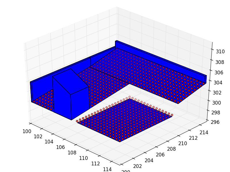
As we have seen, it is very easy to transform a whole space by applying only a single matrix operation and reconstructing it later. I encourage you to create and share the transformations that you require for your applications. Due to this package was created with the shading simulations idea in mind, it may lack of complex transformations. Anyway, more transformations, like stretch, will be added in the future.
photo
The photo’s documentation is quite extense (maybe too much) so I refer to it for the explanation. I am going to extract only this part:
In short, this methods answer “How would the Space look in a photograph taken from an arbitrary direction in cylindrical perpective?”
That is, what is the vision of the Sun from an arbitrary direction? Let’s have a look:
In [10]: poly_hole_points = space.photo((-np.pi/4, np.pi/4), True)  # Oblique

In [11]: poly_hole_points = space.photo((0, np.pi/2), True)  # Zenital

Next tutorial: PiP and Classify tutorial