Back to Guide
PiP and Classify tutorial
Both .pip() and .classify() use the Point-in-Polygon algorithm available in
matplotlib.path.Path.contains_points(). The reason why I’ve created these
methods is to wrap around the matplotlib’s algorithm is because, although it is
actually quite fast, it does not take into account the problem context
(obviously).
pyny3d uses (and abuses) this algorithm to compute shading, among other
secondary processes: usually there are multiple Polygons and a lot of
points in this calculations and if the matplotlib’s version of this algorithm
were used without modifications, it would check whether each point is in or out
each Polygon, this resulting in a very heavy process. What .pip() and
.classify() bring to the table is that they sort the points and the
Polygons bounding boxes by their positions in the cartesian plane before the
calculation starts. With these elements already sorted, it is possible to slice
the space and isolate a small portion of it and locally solve the
Point-in-Polygon algorithm for each Polygon.
We are going to generate a set of points in a mesh and a random set of polygons in z=0. To do the second we are going to use the Voronoi discretization algorithm available in scipy.spatial:
import numpy as np
from scipy.spatial import Voronoi
import pyny3d.geoms as pyny
from pyny3d.utils import sort_numpy
import matplotlib.pyplot as plt

def plot_limits(ax):
    """
    Set the x and y limits of a plot from 0 to 1.
    """
    ax.set_xlim(left=0, right=1)
    ax.set_ylim(bottom=0, top=1)

np.random.seed(seed=3)

# Points (mesh)
n = 50
x1 = np.linspace(0, 1, n)
y1 = np.linspace(0, 1, n)
x1, y1 = np.meshgrid(x1, y1)
points = np.array([x1.ravel(), y1.ravel()]).T

# Surface and Polygon
p = 30
centers = np.random.rand(p, 2)
vor = Voronoi(centers)
## Looking for finite regions (polygons)
polygons_list = []
for vertices in vor.regions[1:]:
    if len(vertices) < 3: continue
    if min(vertices) == -1: continue
    vert = vor.vertices[vertices]
    if vert.max() < 1 and vert.min() > 0:
        polygons_list.append(pyny.Polygon(vert))
## Declaring pyny objects
surface = pyny.Surface(polygons_list)
polygon = surface[0]

# Viz
## Polygon
ax = polygon.plot2d(alpha=0.5, ret=True)
plot_limits(ax)
## Surface
ax = surface.plot2d(alpha=0.5, ret=True)
plot_limits(ax)
## Points
fig = plt.figure()
ax = fig.add_subplot(111)
ax.scatter(points[:, 0], points[:, 1], c='r', s=15, alpha=0.7)
plot_limits(ax)
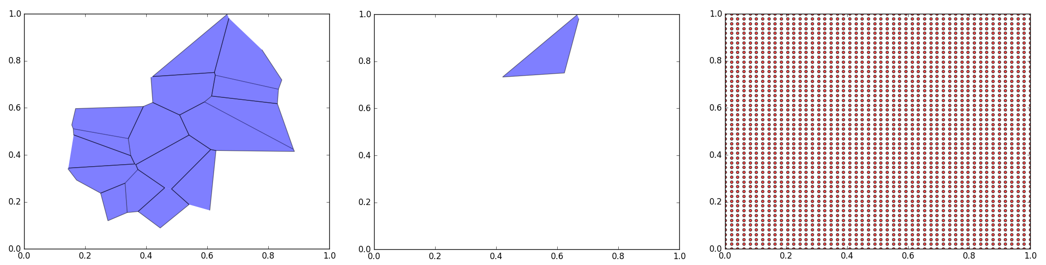
Note that the Polygons have been generated randomly
pip
In practical terms, this method is exactly the same as matplotlib.path.Path.contains_points(). The only change is that it is necessary to have the points previously sorted. We can specify which is the sorted column with the sorted_col argument.
The matplotlib’s version for polygon and points is as follows:
# PiP
## matplotlib's pip
polygon_path = polygon.get_path()
points_in_polygon = points[polygon_path.contains_points(points)]
### Viz
ax = polygon.plot2d(alpha=0.3, ret=True)
ax.scatter(points_in_polygon[:, 0], points_in_polygon[:, 1], c='r', s=25, alpha=0.9)
ax.scatter(points[:, 0], points[:, 1], c='c', s=25, alpha=0.3)
plot_limits(ax)
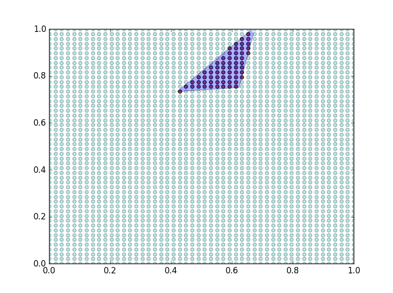
Points in red are inside the polygon while points in cyan are outside
The pyny3d’s pip version produce the same output:
## pyny3d's pip
points_sorted = sort_numpy(points, col=0, order_back=False)
polygon.lock()
points_in_polygon = points_sorted[polygon.pip(points_sorted, sorted_col=0)]
### Viz
ax = polygon.plot2d(alpha=0.3, ret=True)
ax.scatter(points_in_polygon[:, 0], points_in_polygon[:, 1], c='r', s=25, alpha=0.9)
ax.scatter(points[:, 0], points[:, 1], c='c', s=25, alpha=0.3)
plot_limits(ax)
As we will see later in this section, the big difference here is that we can speed up this kind of operations by grouping some steps.
In this case, it would not be necessary to sort the set of points because
the numpy’s meshgrid() function left the output already sorted by the
second column (the y value). Due to most of the time the points are generated
through that function, the default value for sorted_col is 1. In the last
example it would be equivalent (and faster) just to write:
polygon.lock()
points_in_polygon = points[polygon.pip(points)]
classify
It calculates the belonging relationship between the polygons in the Surface and a set of points. That is, given a set of Polygons, grouped in a Surface, and a set of points it computes inside of which polygon is each point. As the rest of the similar methods, everything happens in the z=0 projection of the objects.
For a better understanding, I can tell you that pyny3d uses this method to generate the Solar Horizont data projections where given a discretization of the Sun positions for a year and a data time series with thousands of samples with the form of (azimuth, zenit, value) it has to classify all the samples in the appropriate Polygon:
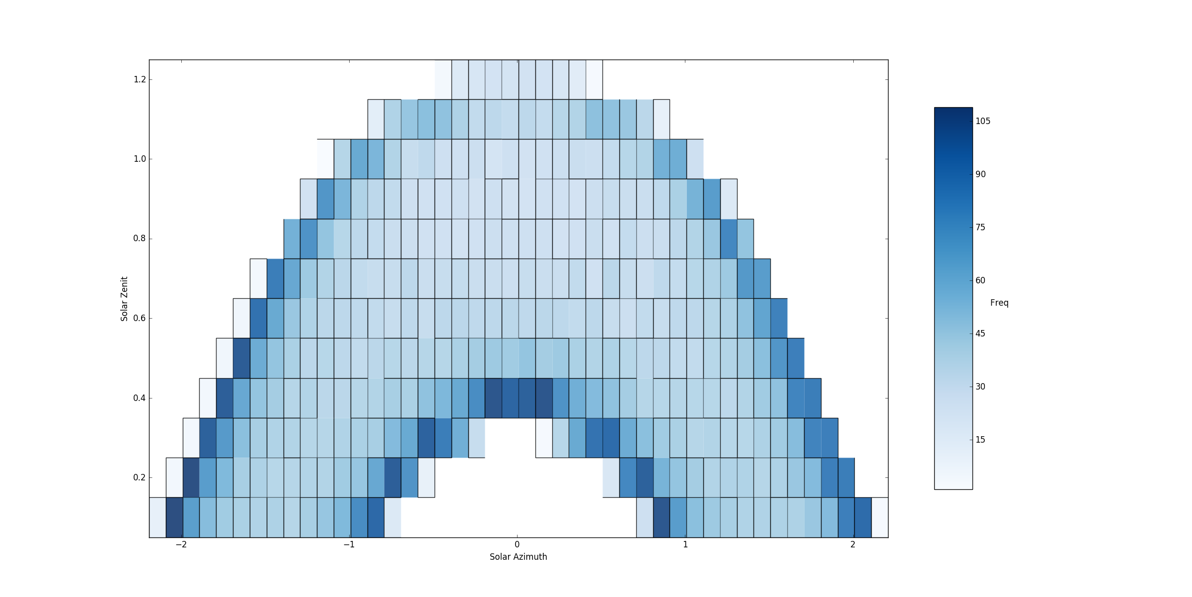
In this Surface there are more than 320 polygons and more than 8500 points have been classified. The value of each point is 1 so the result of the sum for all the points in each polygon is its frequence
Time now for our little example with the points and Surface defined before:
# Classify
mapping = surface.classify(points, edge=True, col=0, already_sorted=False)
## Viz
points_out = points[mapping == -1]
mapping_in = mapping[mapping != -1]
points_in = points[mapping != -1]
ax = surface.plot2d('c', alpha=0.1, ret=True)
ax.scatter(points_in[:, 0], points_in[:, 1], c=mapping_in, cmap='nipy_spectral', s=20)
ax.scatter(points_out[:, 0], points_out[:, 1], c='w', s=20, alpha=0.25)
plot_limits(ax)
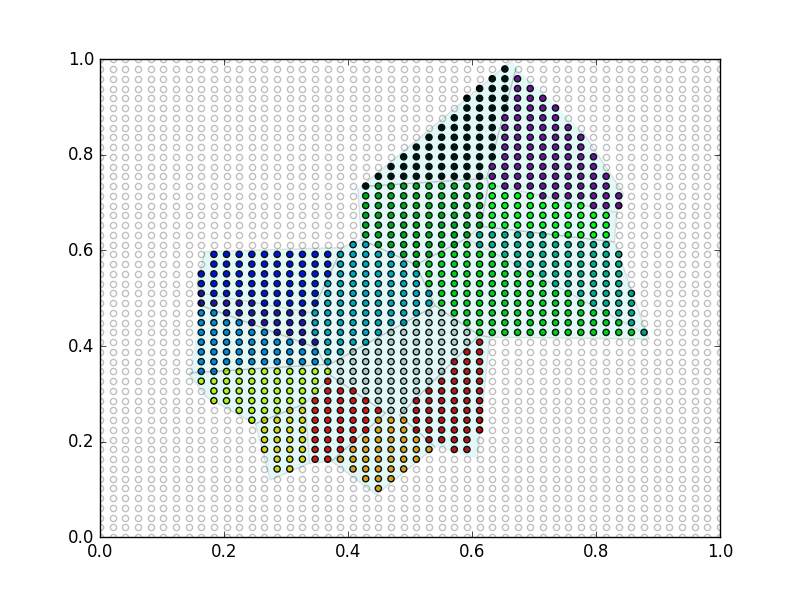
Points in transparent white are those outside polygons (they have a -1 value in ``mapping``). Points in color have been classified and represeted depending on the polygon they belong
As you probably have appreciated, there is no need for sort the points in this
case, it is possible to tell to the method that that already_sorted=False.
Indeed, .classify() also locks the Surface for you. So, why I have to
do it manually in .pip()?
The answer is that .pip() is massively abused in the core of the shading
simulation and adding verifications, locks and sortings would affect
considerably the performance of the pyny3d’s shadows module. On the other
side, although .classify(), is also used in some important parts of the
code, adding some automatic verifications for making our life easier is not
so bad.
As before, we already have the points sorted by the y column so, it would be the same (but faster) to write:
mapping = surface.classify(points, edge=True, col=1, already_sorted=True)
Performance
pip
For a single polygon, the difference between matplotlib’s .contains_points()
and pyny3d’s .pip() is not so great, but it still exists. The main
question here is if it is worth to sort the points and to lock the polygon or
if it is faster just to use .contains_points() directly. The answer will
depend on the capacity of the problem to be grouped, that is, if your problem
has multiple polygons and a lot of points but those are already sorted it is
possible that you can speed up the execution because you only have to lock
the polygons once. However, if you have a dynamic problem with unpredictable
sets of points and polygons try to keep everything in order is probably a waste
of time.
Here we have a comparison between the three posibilities described:
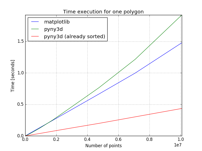
The pyny3d’s execution includes sorting the points and locking the polygon while the “already sorted” version do not include any of those
To illustrate this, I can tell that the whole pyny3d’s shading process
decreased its time investement by half when I replaced the general matplotlib’s
.contains_points() to the more specialised pyny3d’s .pip().
classify
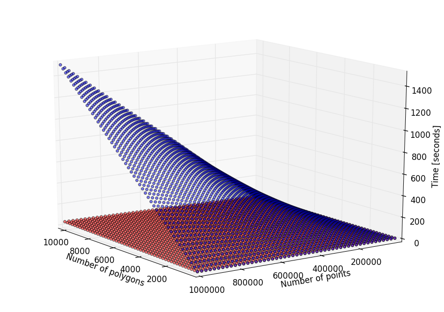
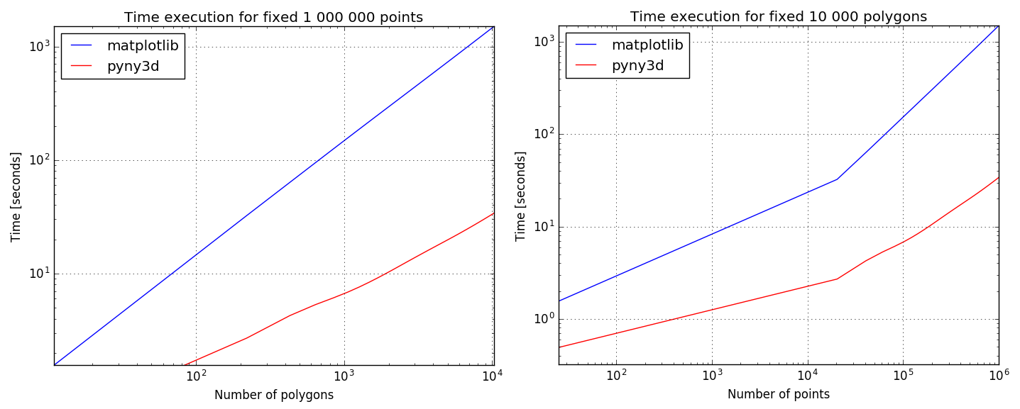
If your problem is simple and it has few points I recommend you to use the matplotlib’s algorithm because it is simpler. However, if you have thousands of points and polygons you should take a look to the following chart:
Performance comparison: matplotlib’s ``.contains_points()`` execution time (in blue) and pyny3d’s ``.classify()`` execution time (in red).
As I remarked before, for few points or polygons the execution time is
very similar but, as we add more elements, the matplotlib’s version gets much
slower than the pyny3d’s. This is because of the previous sorting of
the elements: while .contains_points() is asking each point-polygon
combination for their relationship, .classify() only asks the points which
are known to be inside the local bounding box of the corresponding polygon.
Note
Remember that if you are going to use pyny3d with a lot of
polygons and you are completely sure that the are well defined (like
this case with scipy.spatial.Voronoi) it is possible that you want to
remove the ccw forced verification by setting
pyny.Polygon.verify = False at the start of your code. This will
considerably speed up the process.
Next tutorial: Basic shading tutorial