1. QuickStart
Contents
1.1. Reading data into a dataframe
An example of data file is provided in the package. It contains a YEAST data set with some metadata and measurements for 57 peptides (23 proteins). Let us read it with MSDAS and the MassSpecReader class
>>> from msdas import *
>>> r = MassSpecReader(get_yeast_small_data())
The data is stored in a dataframe df. One can for instance obtain the list of Proteins, Peptide Sequences and Phosphorylation site locations (Psite) as follows:
r.df[['Protein', 'Sequence', 'Psite']]
The dataframe is a data structure from the Pandas library. We will not cover its usage but we strongly advice the reader to look at the Pandas library documentation. Meanwhile, you may want to know a couple of simple manipulations before going on with the MSDAS documentation.
The entire data set is stored in r.df, which is a dataframe with columns and rows. The column names are stored in
r.df.columns
The row names are stored in index:
r.df.index
In this example, the first index is the number 0 and the first column name is called Protein. The following commands are equivalent and return the name of the Protein contained in the first row (with index 0):
r.df.ix[0,'Protein']
r.df.ix[0,0]
r.df.Protein[0]
There are getters than ease access to part of the dataframe. You can extract the data where protein is DIG1 for instance by typing:
r['DIG1']
If you know the psite string, you can even refine the search as follows:
r['DIG1', 'S142']
1.2. Conventions
Let us now spend some time on the input data set and the expected format.
1.2.1. Expected column names in input CSV files
MS-DAS provides tools to read individual CSV files that contain Mass Spectrometry data measurements. However, we do not support existing format or provide any format converter.
The expected format is a CSV file. The first row must be a header with at least the following compulsary names:
- Protein: a uniprot protein name without the _species appended. Ideally it should be a protein name. This column is going to be used to retrieve entry and entry name from uniprot. So, it could also be a gene name.
- Psite: a list of psites where measurement was made. See Psites section for the format.
- Sequence: the peptide sequence. If not provided, populated using the Sequence_Phospho (see next item)
- Sequence_Phospho: the peptide sequence with the Phospho tag to indicate the p-site positions. See section on Sequence here below.
Other optional recognised column names are:
- Entry: uniprot protein name
- Entry_name: uniprot entry names
- Identifier: this is going to be overwritten internally and is the concatentation of Protein and Psite column.
All other columns are read and there is no yet any convention on their names but we could recommend to start all measurements names with the X: tag.
The 7 keywords (Protein, Sequence, ...) are considered to be metadata. All other columns are considered to be measurements. The main dataframe df is a read-write dataframe that contains all metadata and measurements. read-only access to the metadata and the measurements are eased by 2 dataframes named metadata and measurements. The latter is handy to compute statistics. Indeed the mixed of measurements and metadata prevent such manipulation with the main dataframe df.
So, for instance to get the max over all rows in the measurements, you would type:
r.measurements.max(axis=1)
1.2.2. Sequence and Sequence_Phospho column
By Sequence, we mean Sequence of the peptide. 2 column names are accepted:
- Sequence: the raw peptide sequence e.g. GGSSKK
- Sequence_Phospho: the peptide sequence with tag that indicate the loation of the phosphorylation. e.g. GG(Phospho)SSKK
The latter is required. The former if not provided, is rebuilt from the Sequence_Phospho automatically.
1.2.3. Psite column
Psites are encoded as follows. If there is more than 1 psite, we have an AND relation, which is encoded with the “^” character. If there is an ambiguity regarding the position of a site, then this is an OR relation encoded with the “+” character.
Let us consider the following peptide sequence GGSSKK with 2 phosphorylation sites:
GG(Phospho)SS(Phospho)KK
This syntax means that are 2 Psites G at position 2 and S at position 4. The psite name is then encoded as:
G2^S4
However, if there is an ambiguity on the position of G, then it can be coded as follow:
G1+G2^S4
which means there there are 2 phosphorylations: one on S4 and one on G a position 1 or maybe 2.
The tag (Phospho) is placed after the letter:
GG(Phospho)
means Phospho at location 2. The following is incorrect:
(Phospho)GG
See references of msdas.psites.PSites for details.
1.2.4. Replicates
Columns that have the same names are considered replicates. Nevertheless, once read, they have different names in the column names of the dataframe. For instance, a CSV files that contains 3 columns named identically as t0, will have new names t0, t0.1 and t0.2.
1.3. Read a simple data set
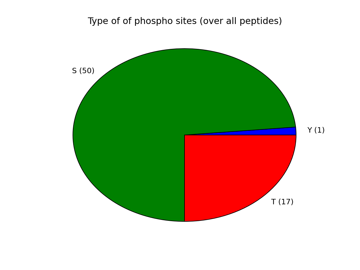
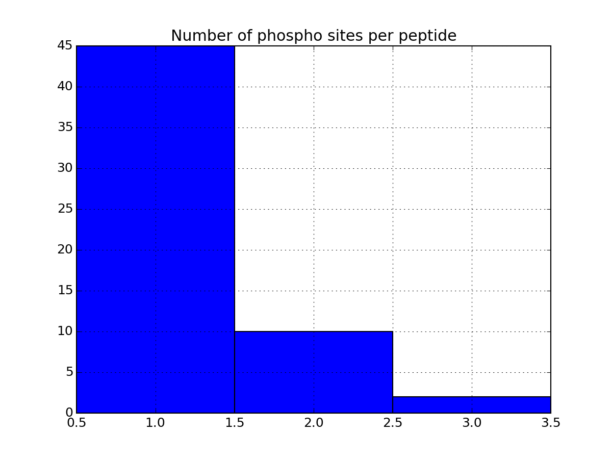
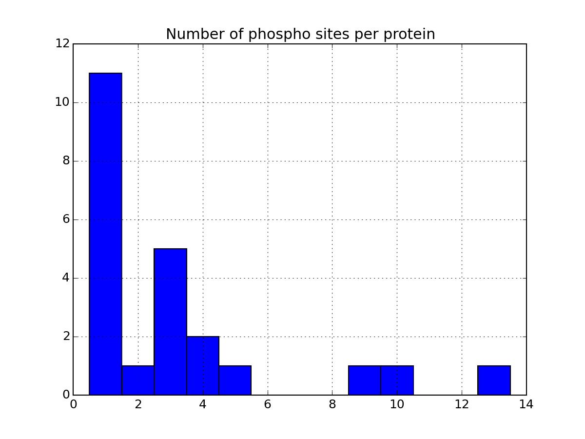
Let us now come back to the data. Once a file has been read with MassSpecReader class, you can have a look at basic figures about the phospho sites:
from msdas import readers, yeast
filename = yeast.get_yeast_filenames()[0]
r = readers.MassSpecReader(filename)
r.plot_phospho_stats()

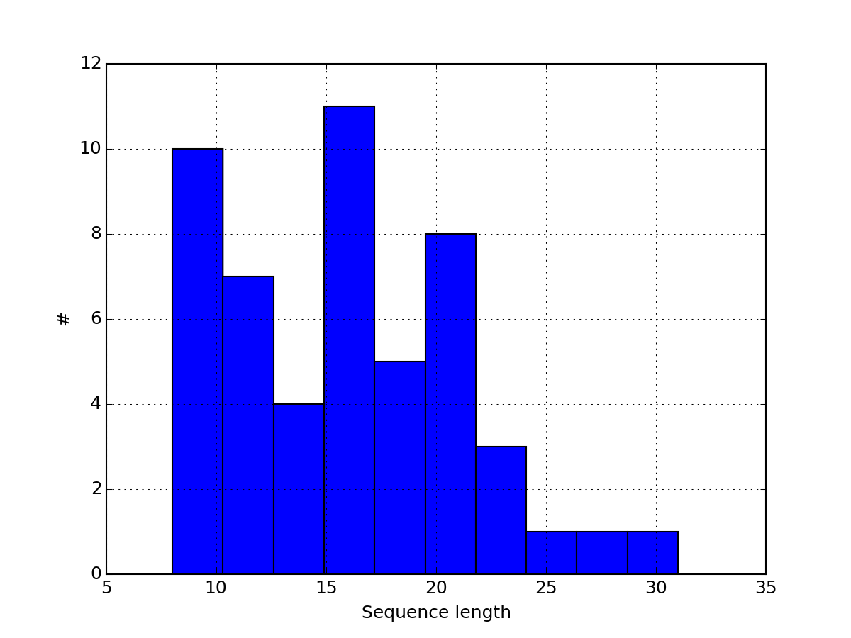
or histogram of the peptide sequence length:
from msdas import *
r = MassSpecReader(get_yeast_filenames()[0])
r.hist_peptide_sequence_length()
(Source code, png, pdf)
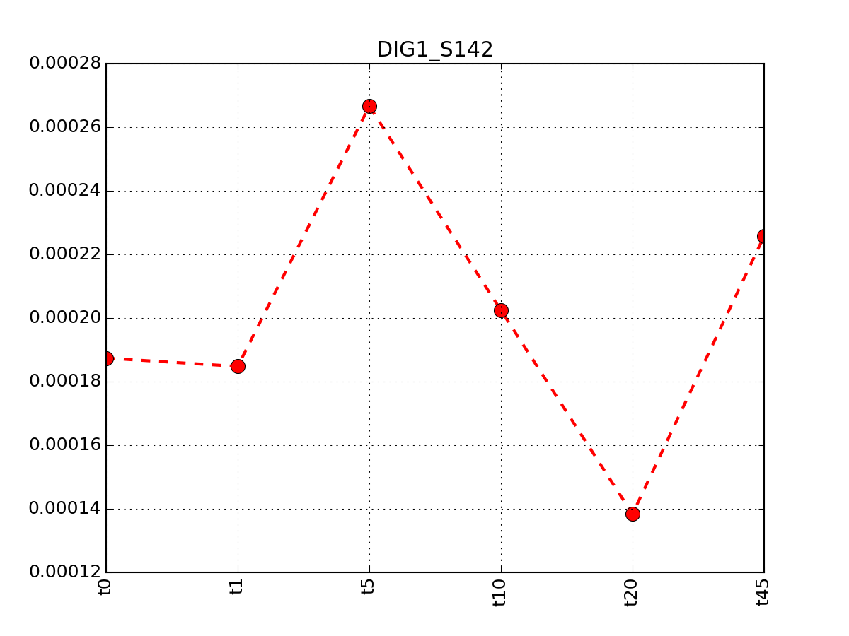
You can look at the data by row:
from msdas import *
r = MassSpecReader(get_yeast_filenames()[0])
r.plot_timeseries("DIG1_S142")
(Source code, png, pdf)

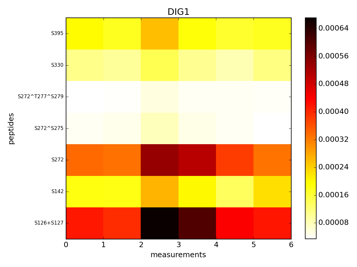
It returns a dataframe with all rows having DIG1 protein. This dataframe can be shown in a color plot:
from msdas import *
r = MassSpecReader(get_yeast_filenames()[0])
r.pcolor("DIG1", tag="t")
(Source code, png, pdf)

Here, tag set to a is the prefix of the measurements.
1.4. Read several files: the alignment class.
The msdas.readers.MassSpecReader class shown above is the core function used to read data sets. As shown above, you can plot some basic figures. Besides, you can perform some cleaning up of the data (e.g., merging of rows with same peptides).
However, you may have several files to read, in which case, they need to be assemble into a single file. For this purpose, you should use the msdas.alignment.MassSpecAlignmentYeast.
Here is an example where the MassSpecAlignmentYeasy class actually reads 6 data files corresponding to 6 different experiments. Once read, the data is gathered in the attribute called df, which can easily converted to a msdas.readers.MassSpecReader instance:
>>> from msdas import *
>>> m = MassSpecAlignmentYeast(get_yeast_filenames(), mode="yeast")
>>> # equivalent to
>>> m = MassSpecAlignmentYeast(yeast.get_yeast_filenames())

>>> r = MassSpecReader(m.df)
>>> r.to_csv("test.csv")
1.4.1. Annotations
The input may file or may not contain information about uniprot entries (Entry, Entry_names). If not provided, you can use the module msdas.annotations.
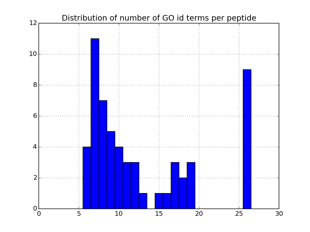
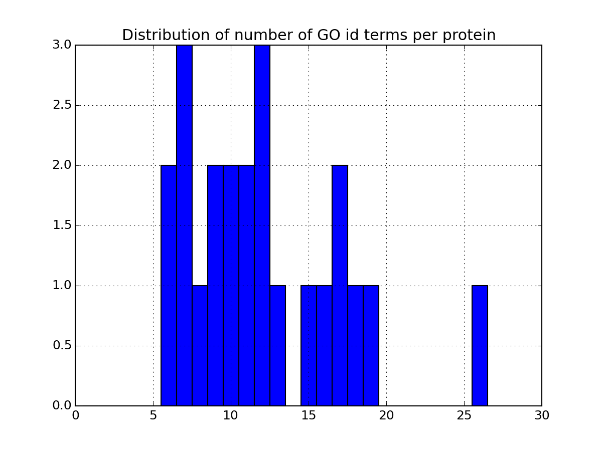
There are many more plotting to describe the data. Some are based solely on your data. Some others requires the parameter annotations to be set to True in the code above. If you set it to True, the code will indeed query information for each protein found in the dataframe. This can be slow so once you have set it to True and all annotations have been downloaded, we recommend you to save the relevant data in a file so to to load it next time (see code below). Once annotations are loaded, you will have access to more functionalities. As an exmaple, the following code plots the most relevant GO terms found in the data (each protein has a number of go terms that can be found in the attribute annotations:
>>> from msdas import alignment, annotations, yeast
>>> m = alignment.MassSpecAlignmentYeast(yeast.get_yeast_filenames())
>>> a = annotations.Annotations(m, "YEAST")
>>> a.get_uniprot_entries()
>>> a.set_annotations()
>>> a.plot_goid_histogram()
Annotations can take a while to load. You can save the results for later:
>>> from msdas import alignment, yeast
>>> m = alignment.MassSpecAlignment(yeast.get_yeast_filenames(), mode="yeast")
>>> a = annotations.Annotations(m, "YEAST")
>>> a.get_uniprot_entries()
>>> a.set_annotations()
>>> a.to_pickle("small")
>>> a.to_csv("dataframe.csv") # saves the dataframe with UniProt Entries and Entry_names
1.5. Debugging and verbosity
We recommend to use MSDAS with verbose set on. The way the software is designed is that all classes have a level of verbosity set with the verbose argument when you create an object.
You can set it to True to have more information. However, there are different level of verbosity. The verbose parameter can be one of:
- DEBUG
- INFO (same as True)
- WARNING
- ERROR (same as False)
DEBUG mode shows all message. INFO show all message except DEBUG. WARNING shows WARNINGs and ERRORS. Finally, ERRORs shows only error messages.
1.6. More about manipulating the dataframe
Once we have a MassSpecMerger object (variable yeast above), we can look at some clustering of the protein per peptides or over a protein.
The yeast instance created above contains all data inside a dataframe called df. This dataframe is used as the common data structure in other classes available inside MS-DAS package.
You can get the size of the dataframe as follows:
>>> m.df.shape
(57, 43)
That is 57 peptides measured and 43 columns. The columns content is given by:
>>> m.df.columns
Index([u'Protein', u'Psite', u'Sequence', u'a0_t0', u'a0_t1', u'a0_t5',
u'a0_t10', u'a0_t20', u'a0_t45', u'a1_t0', u'a1_t1', u'a1_t5', u'a1_t10',
u'a1_t20', u'a1_t45', u'a5_t0', u'a5_t1', u'a5_t5', u'a5_t10', u'a5_t20',
u'a5_t45', u'a10_t0', u'a10_t1', u'a10_t5', u'a10_t10', u'a10_t20', u'a10_t45',
u'a20_t0', u'a20_t1', u'a20_t5', u'a20_t10', u'a20_t20', u'a20_t45', u'a45_t0',
u'a45_t1', u'a45_t5', u'a45_t10', u'a45_t20', u'a45_t45', u'Sequence_original',
u'UniProt_entry', u'GOid', u'GOname'], dtype='object')
Where Protein is the protein name found in the original CSV file, Psite is a protein name appended with psites, Sequence is the peptide sequence (cleanup). Uniprot_entry is the unique uniprot entry given by bioservices/uniprot and GOid/GOname may be populated with bioesrvices/quickgo GO terms.
Other entries (e.g., a0_t45) are measurements found in the yeast CSV files.
More about dataframe manipulation can be found on Pandas website itself.
One nice feature about the dataframe is to be able to group by a specific column (e.g. Protein). Here is a quick example that could be handy:
>>> m.df.groupby("Protein")
>>> df_grouped = m.df.groupby("Protein")
>>> df_grouped.groups
{'DIG1': [0, 1, 2, 3, 4, 5, 6],
'DIG2': [7, 8, 9],
'FAR1': [10],
'FPS1': [11],
'FUS3': [12, 13],
...
Number are the indices of the dataframe (indices correpond to rows in Pandas terminology). So, you can now extract from the original dataframe (or df_grouped), only the row corresponding to a given protein:
>>> m.df.ix[df_grouped.groups['PBS2']]
   Protein      Psite                         Sequence     a0_t0     a0_t1
21    PBS2  PBS2_S248                 TAQQPQQFAPSPSNKK  0.000147  0.000177
22    PBS2  PBS2_S269  SNPGSLINGVQSTSTSSSTEGPHDTVGTTPR  0.000054  0.000046
23    PBS2   PBS2_S68             SASVGSNQSEQDKGSSQSPK  0.000019  0.000019
Note
to access to a row, use yeast.df.ix[index_row]. To access to the column Protein, type yeast.df[‘Protein’]
1.7. Clustering of peptides
Let now now come back to the clustering. We start again from entire data set:
from msdas import readers, clustering, yeast
filename = yeast.get_yeast_small_data()
y = readers.MassSpecReader(filename)
# create a MSclustering instance
and create a clustering instance:
# it will ease the access to the time measurements only
c = clustering.MSClustering(y, mode="YEAST")
The second argument (mode=”yeast”) is compulsary. The clustering object created contains the original dataframe (df) and methods to perform clustering and visulalise the results. Right now, the only method that is implemented is the affinity propagation method, which can be called as follows:
c.run_affinity_propagation_clustering(preference=-120)
The method returns an object if one required further analysis on the clustering itself (see later) but you can also directly use the clustering object to plot the results:
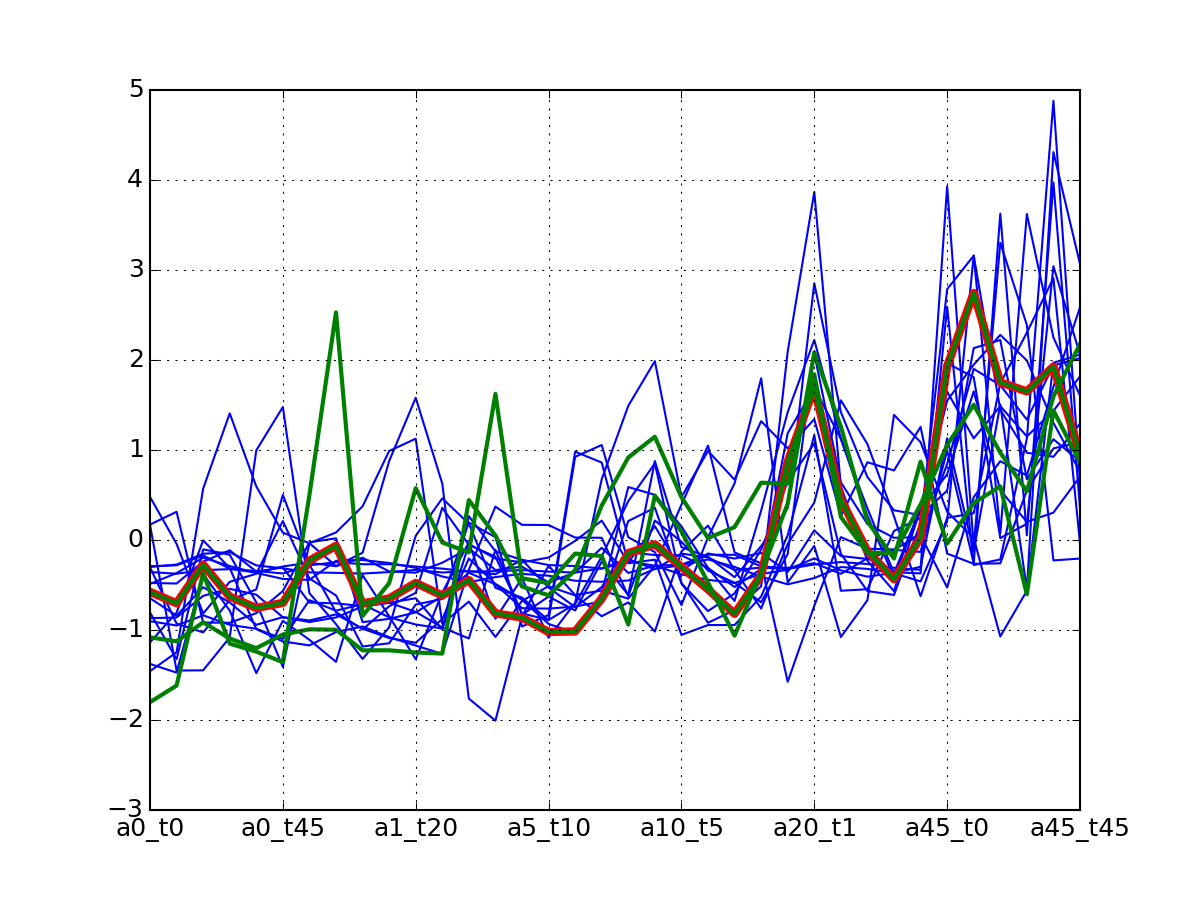
c.plotClusters(legend=False)
and focus on a specific protein:
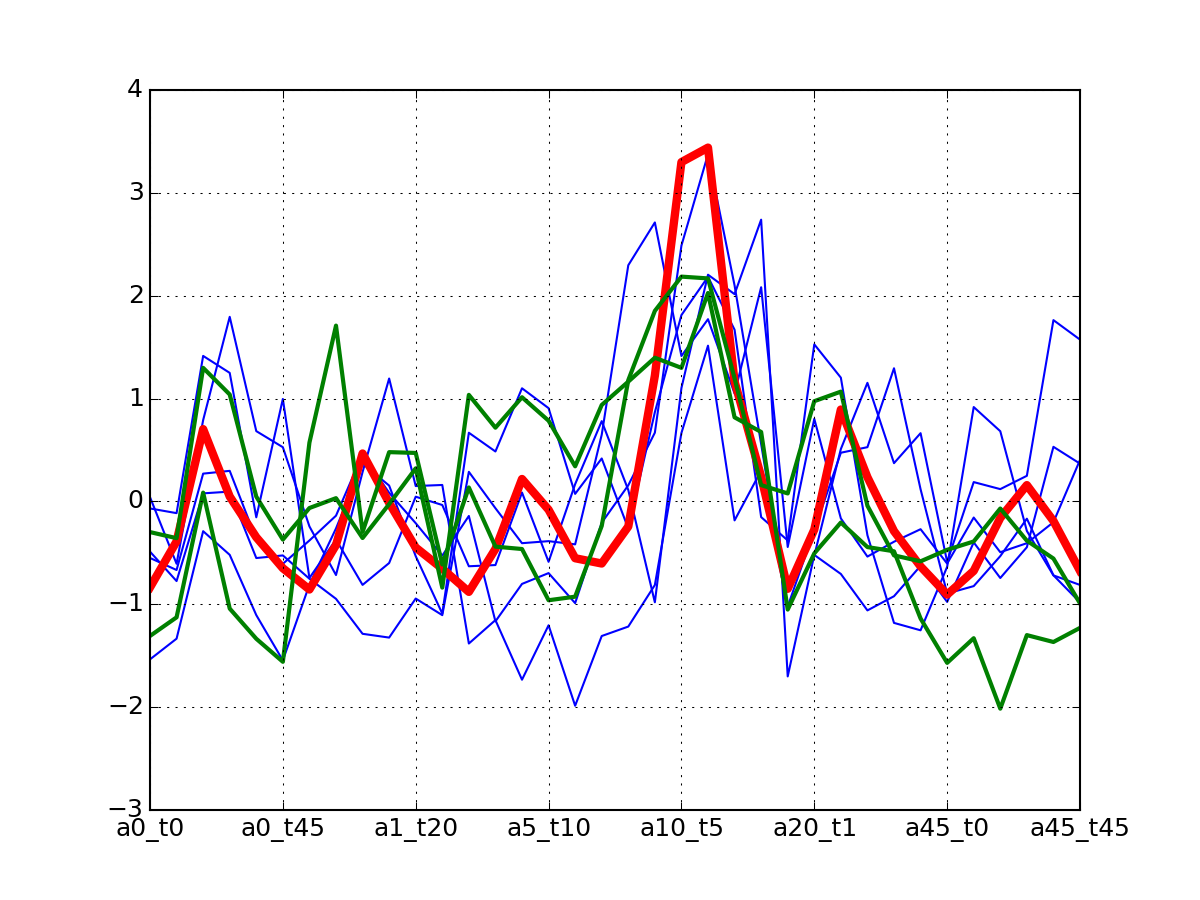
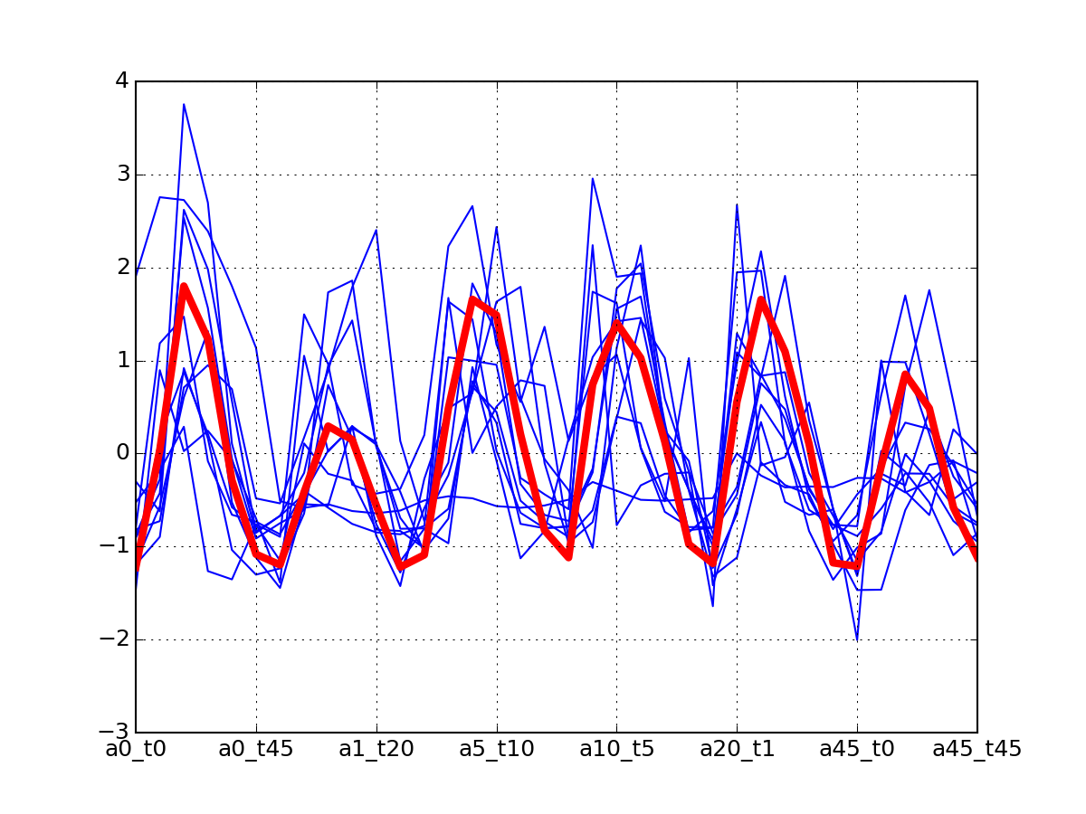
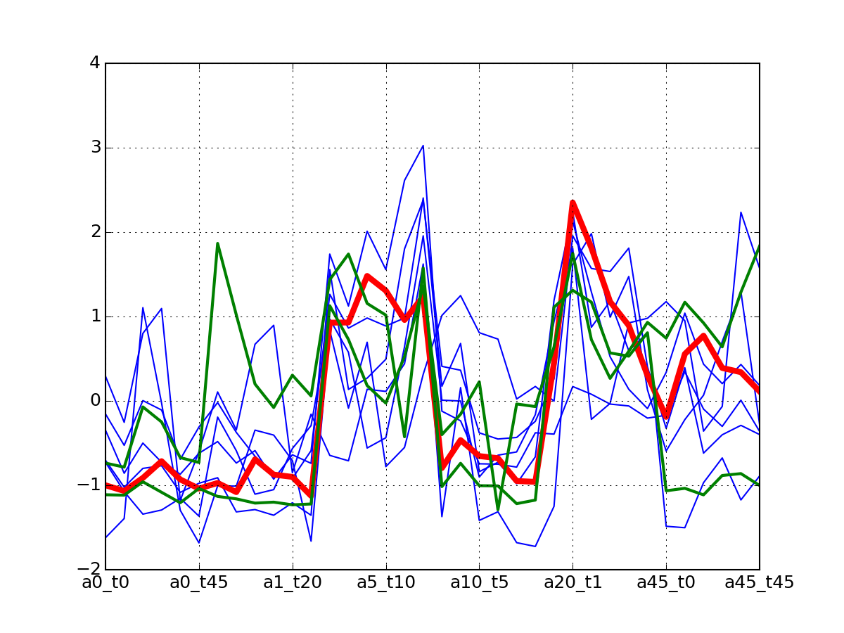
c.plotClusters_and_protein("DIG1", legend=False)
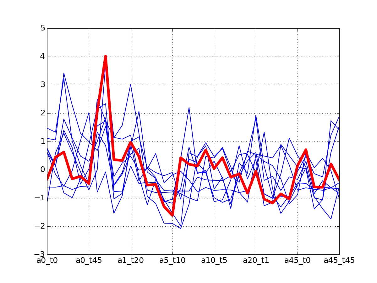
Note
red curve is the examplar, green curves correspond to the protein that has been selected.
When calling the affinity propagation algorithm, the object now what to do (e.g., compute euclidean distance). You can also use directly the Affinity Propagation algorithm as follows:
from msdas import readers, yeast, clustering

y = readers.MassSpecReader(yeast.get_yeast_small_data(), mode="yeast")
# create a MSclustering instance
# it will ease the access to the time measurements only
c = clustering.MSClustering(y)
# some values may have been set to NA, For the affinity propagation
# algorithm, NAs raise errors. So, we need to replace by zero
c.df.fillna(0, inplace=True)

# clustering using AffinityPropagation is used here
af = clustering.Affinity(c.get_group(), method="euclidean")
af.affinity_matrix = af.affinity_matrix.transpose()
af.AffinityPropagation(preference=-120);
af.plotClusters_and_protein("DIG1", legend=False)

