caps.diffusion_estimation.py_tensor_estimation.SecondOrderTensorEstimation
SecondOrderTensorEstimation
- class caps.diffusion_estimation.py_tensor_estimation.SecondOrderTensorEstimation(autoexport_nodes_parameters=True, **kwargs)[source]
Second Order Tensor Estimation
[+show/hide tensor modelisation]
Fit the diffusion tensor model using two strategies:
- Ordinary least suquare fit (fast)
- Quartic decomposition based fit (return positive semi definite tensors)
Get tensor scalar invariant properties: the fractional anisotropy, the mean diffusivity and the Westion shapes coefficients.
![\vec{g}=[g_1,g_2,g_3]](../../../_images/math/f0584edbd5583835931ffa434810920356ece21a.png) the measure direction, the
Stejskal Tanner can be generalized as follows:
the measure direction, the
Stejskal Tanner can be generalized as follows: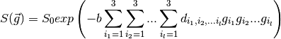
 is the l order tensor components.
The diffusion profile represented by this tensor can be written as follows:
is the l order tensor components.
The diffusion profile represented by this tensor can be written as follows: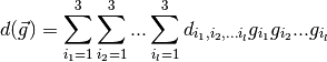
 elements. The full
symmetry property associated with a diffusion tensor reduces the number of
independent components. This property comes from the fact that a diffusion
tensor has to link the different components of a vector to the same scalar
elements. The full
symmetry property associated with a diffusion tensor reduces the number of
independent components. This property comes from the fact that a diffusion
tensor has to link the different components of a vector to the same scalar
 . For instance, when l=2 we have:
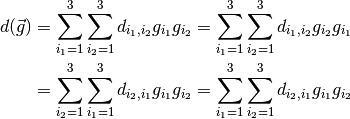
 since it is satisfied
for any vector
since it is satisfied
for any vector  . A similar analysis for a l order tensor gives:
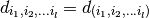
 represents all the possible permutations of
indices. In three dimensions, a symmetric tensor has:
represents all the possible permutations of
indices. In three dimensions, a symmetric tensor has:
 is the number of l-combinations with
repetition of 3 elements), where each element
is the number of l-combinations with
repetition of 3 elements), where each element  (
(![k \in [1,\dots, N_l]](../../../_images/math/711e22c65c190a35479ce6898ce48ca926b7f7a6.png) ) is repeated
) is repeated  times, with:
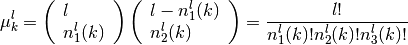
 and
and  are respectivelly the number
of index 1, 2 and 3 that defined the kth independant component of the tensor:
are respectivelly the number
of index 1, 2 and 3 that defined the kth independant component of the tensor:
 . Finally, we can rewrite the
Steskal-Tanner equation:
. Finally, we can rewrite the
Steskal-Tanner equation: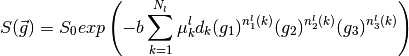
Inputs
[Mandatory]
bvals_file: a file name (mandatory)
the the diffusion b-values
|
bvecs_file: a file name (mandatory)
the the diffusion b-vectors
|
dwi_file: a file name (mandatory)
an existing diffusion weighted image
|
mask_file: a file name (mandatory)
a mask image
|
reference_file: a file name (mandatory)
the referecne b=0 image
|
[Optional]
Outputs
eigen_values_file: a file name
the name of the output eigen values file
|
eigen_vectors_file: a file name
the name of the output eigen vectors file
|
fractional_anisotropy_file: a file name
the name of the output fa file
|
linearity_file: a file name
the name of the fie that contains the linerity coefficients
|
mean_diffusivity_file: a file name
the name of the output md file
|
planarity_file: a file name
the name of the fie that contains the planarity coefficients
|
sphericity_file: a file name
the name of the fie that contains the sphericity coefficients
|
tensor_file: any value
|
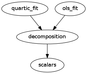
Pipeline schema