Overview and Tutorial

The pymodelfit module contains objects and functions for fitting data to models as well as calculations and estimates from these models. The available fitting algorithms are those from scipy.optimize or the PyMC .

The aim of these classes are mostly for easily and quickly generating a range of models. There are classes in core for various dimensionalities, and helper classes to make it trivial to implement one of these classes. For example, most models can be implemented as a subclass with only a single additional function describing the model itself. Further, the module includes a model registry to easily access the builtin models and any others the user wishes to implement.

Module Organization

The pymodelfit package is composed of two submodules that are both imported into the main module. The first, core contains the classes and functions that structure and do most of the work of the models. The second, builtins contains a default set of models. There are two additional modules that contain GUIs for interactive model-fitting. For single 1D models, the fitgui module contains the gui, while for a multi-variable fit, the multifitgui can fit multiple simultaneous 1D relations and display them in 3D.

Note

Everything in the core and builtins modules are present in the pymodelfit module, and hence can be accessed from there. For example, pymodelfit.core.FunctionModel and pymodelfit.FunctionModel are different names for the same class. The second form is recommended for consistency and brevity.

Tutorial/Examples

The basic idea of pymodelfit is to use either a custom-defined model (see example below), or one of the builtin models (in builtins) to represent a model and its associated parameters, which can then be fit to a supplied dataset, providing the best-fit parameters. While the default fitting technique (the Levenberg-Marquardt algorithm) is fairly robust and standard, pymodelfit provides a number of ways to customize fitting methods for a given model, providing both power and flexibility.

pymodelfit can support different dimensionality of models (e.g. 3D vector-to-scalar, 3D vector-to-3D vector, 2D vector-to-scalar, etc.), but the most common and simplest application is for a 1D model (e.g. scalar-to-scalar), and hence the examples below are geared towards that intent. In general, higher-dimensional models follow smilar pattern, but the arrays accepted and returned must be the correct dimensionality. See the reference for the base classes of higher-dimensional models (e.g. FunctionModel2DScalar) for details.

Accessing and Creating Models

The first crucial step is to generate a new copy (instance) of a model. The simplest way is to simply use the class of the model itself as you would any other python object:

>>> from pymodelfit import LinearModel
>>> linmod = LinearModel(m=1.25,b=3)

This thus creates a model for a linear relation with a slope of 1.25 and y-intercept of 3.

Alternatively, to access a builtin model or any custom models that have been registered (as described below) by name, the get_model_instance() function is the appropriate technique:

>>> linmod = get_model_instance('linear')
>>> linmod.m = 1.25
>>> linmod.b = 3
>>> linmod([0,1,2])
array([ 3.  ,  4.25,  5.5 ])
>>> linmod.__class__
<class 'pymodelfit.builtins.LinearModel'>

A list of available models can be obtained with the list_models(), and this list can be used to get only models of a specific dimensionality. The two examples below are for scalar->scalar models, and 2D vector->scalar models):

>>> list_models(baseclass=FunctionModel1D)
['linearinterpolated', 'constant', 'lognormal', 'twoslopediscontinuous',
'interpolatedspline', 'doubleopposedgaussian', 'polynomial',
'uniformknotspline', 'smoothspline', 'maxwellboltzmannspeed', 'quadratic',
'twoslope', 'sin', 'linear', 'twoslopeatan', 'gaussian', 'twopower',
'doublegaussian', 'powerlaw', 'voigt', 'specifiedknotspline',
'uniformcdfknotspline', 'exponential', 'alphabetagamma', 'maxwellboltzmann',
'nearestinterpolated', 'fourier', 'lorentzian']
>>> list_models(baseclass=FunctionModel2DScalar)
['linear2d', 'gaussian2d']

Fitting a Model to Data

With an instance of a model, it is now possible to fit that model to a given data set:

>>> from pymodelfit import LinearModel
>>> linmod = LinearModel()
>>> mf,bf = linmod.fitData(x,y)

This will fit the model to the data that is expected to take in x as an input and output y. The fitData() method minimizes the sum of the squares of the residuals between the data and the model to determine the parameters, and those parameters are stored in the model as m and b, and are also returned as the result of the call to fitData().

Plotting the Model and Data

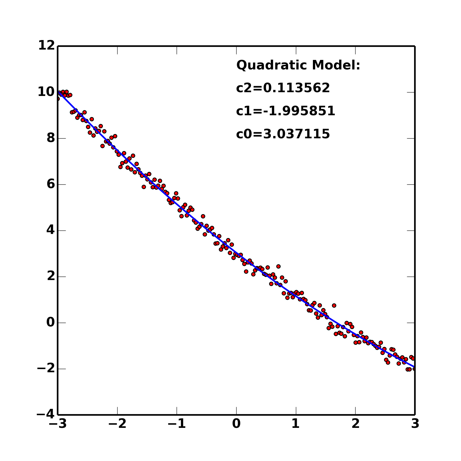
If matplotlib is installed, this dataset and the fitted model can be visualized via the plot() method. This shows both the data (as points) and the best-fit model (the curve). The plot can be customized by providing keywords accepted by the relevant matplotlib plotting functions (see plot() docs for details). This allows publication-quality plots of models and their associated fits.

from numpy import linspace
from numpy.random import randn
from pymodelfit import QuadraticModel
from matplotlib import pyplot as plt

x = linspace(-3,3,200)
y = 0.12*x**2-2*x+3
yr = y + randn(x.size)/4

qm = QuadraticModel()
qm.fitData(x,yr)
qm.plot()
plt.text(0,11,'Quadratic Model:',fontsize=16)
for i,k in enumerate(qm.pardict):
    plt.text(0,10-i,'%s=%f'%(k,qm.pardict[k]),fontsize=16)
plt.show()

(Source code, png, hires.png, pdf)

Creating a Custom Model

Often, you will want to create a model with a functional form that does not match one of the builtin models – perhaps a field-specific form, or a model informed by some expectation of the characterstics oft he input data.

While a custom model can be written by directly subclassing FunctionModel subclasses of appropriate dimensionality, the much easier way is to inherit from one of the models that ends in ‘Auto’:

from pymodelfit import FunctionModel1DAuto
class CuberootLinearModel(FunctionModel1DAuto):
    def f(self,x,a=1,b=5,c=0):
        return a*x**(1/3) + b*x + c

The ‘Auto’ classes take care of assigning the parameter names and defaults based on the signature of the f function. The resulting class in the example above thus represents a mixed cubed-root/linear model, and all of the model-fitting, plotting, and related tools are immediately available simply by doing:

model = CuberootLinearModel()

Many more options are available for specifying additional information about a custom model. These include special fitting functions, descriptions of the ranges over which the models are valid, or suggested names for the model axes. The exact syntax for these options are detailed in the base classes for the relevant models (e.g. FunctionModel1D).

The best source of examples of creating models is the source code of the builtins module. All of the models therein are written exactly as a custom model can be, and show examples of all the available options, including custom fitting methods.

Registering a Custom Model

While the the CuberootLinearModel model from above can be used as-is with standard python class syntax, for it to be visible in other tools for tools like the fitGui interface, it must be registered with pymodelfit using the register_model() function:

from pymodelfit import register_model
register_model(CuberootLinearModel)

The model will now be available in the get_model_class() and get_model_instance() functions under the name ‘cuberootlinear’ (the default name can be changed using the name parameter of register_model()). Thus, the new model will be visible to anything that uses pymodelfit that uses functional models (e.g. the gui module, external packages like astropysics that use models in some places, etc.)

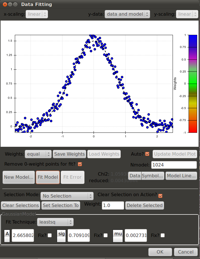
Interactively Fitting a Model With a GUI Interface

A GUI Interface is also included that allows for interactive fitting of a datset to any of the registered models. The details for this interface are given in the description of the module it can be found at Interactive Curve Fitting – GUI Tools.