Tutorial

Solving problem 701

Filename: examples/demo_wave_DWT_deconv.py

The following tutorial shows how to solve problem 701 (compsense.problems.prob701) using the TwIST algorithm (compsense.algorithms.TwIST).

First we need to import the pycompsense package:

>>> import compsense

Then we create the problem object. We can use the default problem settings or change them. Here we use a different noise variance:

>>> P = compsense.problems.prob701(sigma=1e-3)

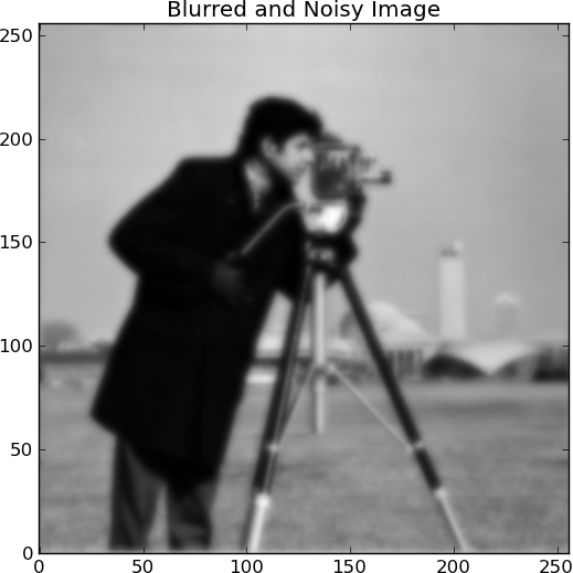
The problem blurs and adds noise to the cameraman.jpg image

We use the TwIST algorithm to solve the following optimization problem

where and (the measured signal, the blurring operator and the sparsifying basis, respectively) are defined by the problem object P. The algorithm object accepts the problem object P and the algorithm parameters:

>>> tau = 0.00005
>>> alg = compsense.algorithms.TwIST(
  ...     P,
  ...     tau,
  ...     stop_criterion=1,
  ...     tolA=1e-3
  ...     )

To solve the problem we need to call the solve method of the algorithm:

>>> x = alg.solve()

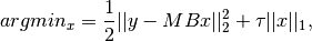
The solution of the problem, x, is the coefficients of the signal in the sparsifying basis. To reconstruct the estimated signal we use the reconstruct method of the problem:

>>> y  = P.reconstruct(x)

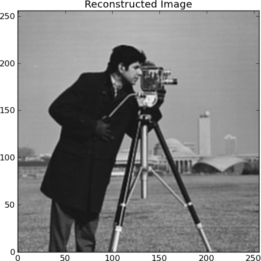
We can also display statics of the algorithm. For example we can display the evolution of the objective of the optimization problem:

>>> plt.figure()
>>> plt.semilogy(alg.times, alg.objectives, lw=2)
>>> plt.title('Evolution of the objective function')
>>> plt.xlabel('CPU time (sec)')
>>> plt.grid(True)

This results in

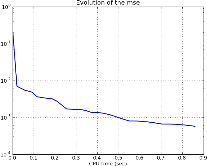
Or we can display the evolution of the mse error of the data term in the optimization problem:

>>> plt.figure()
>>> plt.semilogy(alg.times, alg.mses, lw=2)
>>> plt.title('Evolution of the mse')
>>> plt.xlabel('CPU time (sec)')
>>> plt.grid(True)

This results in

More examples can be found in the source distribution under the examples/ folder.