
By default, the samples try to be as uncorrelated and independent as possible from any other inputs. However, sometimes inputs to have some degree of correlation between them. If it is desired to force a set of variables to have certain correlations, which is not uncommon in real-life situations, this can be done with the correlate function (NOTE: this should be done BEFORE any calculations have taken place in order to work properly).
For example, let’s look at our A Simple Example with inputs x1, x2, and x3:
# The correlation coefficients before adjusting
>>> print correlation_matrix([x1, x2, x3])
[[ 1.          0.00558381  0.01268168]
 [ 0.00558381  1.          0.00250815]
 [ 0.01268168  0.00250815  1.        ]]
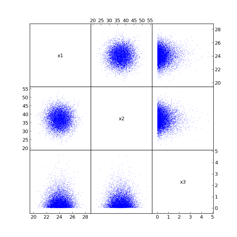
You’ll notice a few things about the correlation matrix. First, the diagonals are all 1.0 (they always are). Second, the matrix is symmetric. Third, the correlation coefficients in the upper and lower triangular parts are relatively small. This is how mcerp is designed.
Here is what the actual samples looks like in a matrix plot form (created using plotcorr([x1, x2, x3], labels=['x1', 'x2', 'x3'])):
Now, let’s say we desire to impose a -0.75 correlation between x1 and x2. Let’s create the desired correlation matrix (note that all diagonal elements should be 1.0):
# The desired correlation coefficient matrix
>>> c = np.array([[  1.0, -0.75, 0.0],
...               [-0.75,   1.0, 0.0],
...               [  0.0,   0.0, 1.0]])
Using the mcerp.correlate function, we can now apply the desired correlation coefficients to our samples to try and force the inputs to be correlated:
# Apply the correlations into the samples (works in-place)
>>> correlate([x1, x2, x3], c)

# Show the new correlation coefficients
>>> print correlation_matrix([x1, x2, x3])
[[  1.00000000e+00  -7.50010477e-01   1.87057576e-03]
 [ -7.50010477e-01   1.00000000e+00   8.53061774e-04]
 [  1.87057576e-03   8.53061774e-04   1.00000000e+00]]
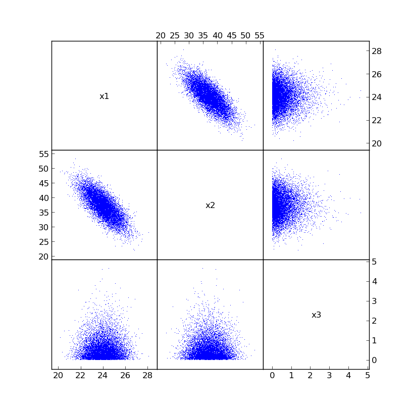
The correlation matrix is roughly what we expected within a few percent. Even the other correlation coefficients are closer to zero than before. If any exceptions appear during this operation, it is likely because the correlation matrix is either not symmetric, not positive-definite, or both.
The newly correlated samples will now look something like:
Now that the inputs’ relations have been modified, let’s check how the output of our stack-up has changed (sometimes the correlations won’t change the output much, but others can change a lot!):
# Z should now be a little different
>>> Z = (x1*x2**2)/(15*(1.5 + x3))
>>> Z.describe
MCERP Uncertain Value:
 > Mean...................  1153.710442
 > Variance...............  97123.3417748
 > Skewness Coefficient...  0.211835225063
 > Kurtosis Coefficient...  2.87618465139
We can also see what adding that correlation did: reduced the mean, reduced the variance, increased the skewness, increased the kurtosis.