Learning the ropes
In the tutorials, we will introduce the PySPH framework in the context of the examples provided. Read this if you are a casual user and want to use the framework as is. If you want to add new functions and capabilities to PySPH, you should read The PySPH framework. If you are new to PySPH however, we highly recommend that you go through this document and the next tutorial (A more detailed tutorial).
Recall that PySPH is a framework for parallel SPH-like simulations in Python. The idea therefore, is to provide a user friendly mechanism to set-up problems while leaving the internal details to the framework. All examples follow the following steps:
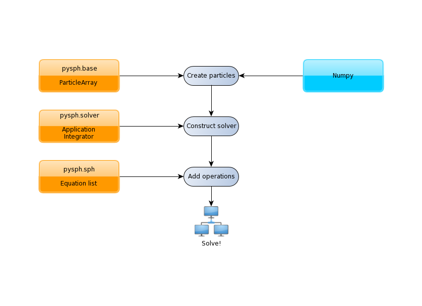
The tutorials address each of the steps in this flowchart for problems with increasing complexity.
The first example we consider is a “patch” test for SPH formulations for incompressible fluids in elliptical_drop.py. This problem simulates the evolution of a 2D circular patch of fluid under the influence of an initial velocity field given by:
The kinematical constraint of incompressibility causes the initially circular patch of fluid to deform into an ellipse such that the volume (area) is conserved. An expression can be derived for this deformation which makes it an ideal test to verify codes.
Imports
Taking a look at the example (see elliptical_drop.py), the first several lines are imports of various modules:
import os
from numpy import array, ones_like, mgrid, sqrt
import numpy as np

from pysph.base.utils import get_particle_array
from pysph.base.kernels import Gaussian

from pysph.solver.application import Application
from pysph.sph.integrator import EPECIntegrator
from pysph.sph.scheme import WCSPHScheme
Note
This is common for most examples and it is worth noting the pattern of the
PySPH imports. Fundamental SPH constructs like the kernel and particle
containers are imported from the base subpackage. The framework
related objects like the solver and integrator are imported from the
solver subpackage. Finally, we import from the sph subpackage, the
physics related part for this problem.
Functions for loading/generating the particles
The code begins with a few functions related to obtaining the exact solution for the given problem which is used for comparing the computed solution.
A single new class called EllipticalDrop which derives from
pysph.solver.application.Application is defined. There are several
methods implemented on this class:
initialize: lets users specify any parameters of interest relevant to the simulation.create_scheme: lets the user specify thepysph.sph.scheme.Schemeto use to solve the problem. Several standard schemes are already available and can be readily used.create_particles: this method is where one creates the particles to be simulated.post_process: optionally post-process the results generated.
Of these, create_particles and create_scheme are mandatory for without
them SPH would be impossible. The rest (and other methods) are optional. To
see a complete listing of possible methods that one can subclass see
pysph.solver.application.Application.
The create_particles method looks like:
class EllipticalDrop(Application):
    # ...
    def create_particles(self):
        """Create the circular patch of fluid."""
        dx = self.dx
        hdx = self.hdx
        co = self.co
        ro = self.ro
        name = 'fluid'
        x, y = mgrid[-1.05:1.05+1e-4:dx, -1.05:1.05+1e-4:dx]
        x = x.ravel()
        y = y.ravel()

        m = ones_like(x)*dx*dx
        h = ones_like(x)*hdx*dx
        rho = ones_like(x) * ro

        p = ones_like(x) * 1./7.0 * co**2
        cs = ones_like(x) * co

        u = -100*x
        v = 100*y

        # remove particles outside the circle
        indices = []
        for i in range(len(x)):
            if sqrt(x[i]*x[i] + y[i]*y[i]) - 1 > 1e-10:
                indices.append(i)

        pa = get_particle_array(x=x, y=y, m=m, rho=rho, h=h, p=p, u=u, v=v,
                                cs=cs, name=name)
        pa.remove_particles(indices)

        print("Elliptical drop :: %d particles"%(pa.get_number_of_particles()))
        self.scheme.setup_properties([pa])

        return [pa]
The method is used to initialize the particles in Python. In PySPH, we use a
ParticleArray object as a container for particles of a given
species. You can think of a particle species as any homogenous entity in a
simulation. For example, in a two-phase air water flow, a species could be
used to represent each phase. A ParticleArray can be conveniently
created from the command line using NumPy arrays. For example
>>> from pysph.base.utils import get_particle_array
>>> x, y = numpy.mgrid[0:1:0.01, 0:1:0.01]
>>> x = x.ravel(); y = y.ravel()
>>> pa = sph.get_particle_array(x=x, y=y)
would create a ParticleArray, representing a uniform distribution
of particles on a Cartesian lattice in 2D using the helper function
get_particle_array() in the base subpackage. The
get_particle_array_wcsph() is a special version of this suited to
weakly-compressible formulations.
Note
ParticleArrays in PySPH use flattened or one-dimensional arrays.
The ParticleArray is highly convenient, supporting methods for
insertions, deletions and concatenations. In the create_particles
function, we use this convenience to remove a list of particles that fall
outside a circular region:
pa.remove_particles(indices)
where, a list of indices is provided. One could also provide the indices in
the form of a LongArray which, as the name suggests, is an array
of 64 bit integers.
Note
Any one-dimensional (NumPy) array is valid input for PySPH. You can generate this from an external program for solid modelling and load it.
Note
PySPH works with multiple ParticleArrays. This is why we actually return a list in the last line of the get_circular_patch function above.
The create_particles always returns a list of particle arrays even if
there is only one. The method self.scheme.setup_properties automatically
adds any properties needed for the particular scheme being used.
Setting up the PySPH framework
As we move on, we encounter instantiations of the PySPH framework objects.
In this example, the pysph.sph.scheme.WCSPH scheme is created in
the create_scheme method. The WCSPHScheme internally creates other
basic objects needed for the SPH simulation. In this case, the scheme
instance is passed a list of fluid particle array names and an empty list of
solid particle array names. In this case there are no solid boundaries. The
class is also passed a variety of values relevant to the scheme and
simulation. The kernel to be used is created and passed to the
configure_solver method of the scheme. The
pysph.sph.integrator.EPECIntegrator is used to integrate the
particle properties. Various solver related parametes are also setup.
def create_scheme(self):
    s = WCSPHScheme(
        ['fluid'], [], dim=2, rho0=self.ro, c0=self.co,
        h0=self.dx*self.hdx, hdx=self.hdx, gamma=7.0, alpha=0.1, beta=0.0
    )
    kernel = Gaussian(dim=2)
    dt = 5e-6; tf = 0.0076
    s.configure_solver(
        kernel=kernel, integrator_cls=EPECIntegrator, dt=dt, tf=tf,
        adaptive_timestep=True, cfl=0.3, n_damp=50,
        output_at_times=[0.0008, 0.0038]
    )
    return s
As can be seen, various options are configured for the solver, including initial damping etc. The scheme is responsible for:
- setting up the actual equations that describe the interactions between particles (see SPH equations),
- setting up the kernel (SPH Kernels) and integrator (Integrator module) to use for the simulation.
- setting up the Solver (Module solver), which marshalls the entire simulation.
For a more detailed introduction to these aspects of PySPH please read, the
A more detailed tutorial tutorial which provides greater detail on these.
However, by simply creating the WCSPHScheme and creating the particles,
one can simulate the problem.
The astute reader may notice that the EllipticalDrop example is
subclassing the Application. This makes it easy to pass command
line arguments to the solver. It is also important for the seamless parallel
execution of the same example. To appreciate the role of the
Application consider for a moment how might we write a parallel
version of the same example. At some point, we would need some MPI imports and
the particles should be created in a distributed fashion. All this (and more)
is handled through the abstraction of the Application which hides
all this detail from the user.
Running the example
In the last two lines of the example, we instantiate the EllipticalDrop
class and run it:
if __name__ == '__main__':
    app = EllipticalDrop()
    app.run()
There is an additional post_process call in the code which is entirely
optional and will generate some data for comparison with the exact solution.
The Application takes care of creating the particles, creating the
solver, handling command line arguments etc. Many parameters can be
configured via the command line, and these will override any parameters setup
in the respective create_* methods. For example one may do the following
to find out the various options:
$ pysph run elliptical_drop -h
If we run the example without any arguments it will run until a final time of 0.0075 seconds. We can change this example to 0.005 by the following:
$ pysph run elliptical_drop --tf=0.005
When this is run, PySPH will generate Cython code from the equations and
integrators that have been provided, compiles that code and runs the
simulation. This provides a great deal of convenience for the user without
sacrificing performance. The generated code is available in
~/.pysph/source. If the code/equations have not changed, then the code
will not be recompiled. This is all handled automatically without user
intervention. By default, output files will be generated in the directory
elliptical_drop_output.
If we wish to utilize multiple cores we could do:
$ pysph run elliptical_drop --openmp
If we wish to run the code in parallel (and have compiled PySPH with Zoltan and mpi4py) we can do:
$ mpirun -np 4 pysph run elliptical_drop
This will automatically parallelize the run using 4 processors. In this example doing this will only slow it down as the number of particles is extremely small.
Visualizing and post-processing
You can view the data generated by the simulation (after the simulation
is complete or during the simulation) by running the pysph view
command. To view the simulated data you may do:
$ pysph view elliptical_drop_output
If you have Mayavi installed this should show a UI that looks like:
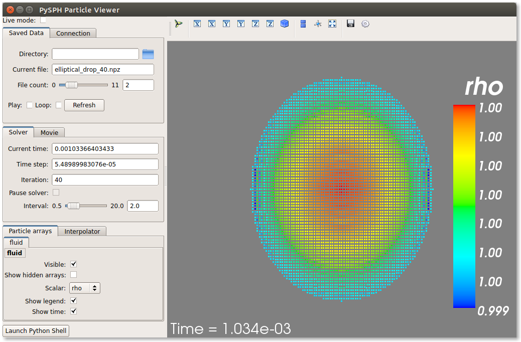
On the user interface, the right side shows the visualized data. On top of it there are several toolbar icons. The left most is the Mayavi logo and clicking on it will present the full Mayavi user interface that can be used to configure any additional details of the visualization.
On the bottom left of the main visualization UI there is a button which has the text “Launch Python Shell”. If one clicks on this, one obtains a full Python interpreter with a few useful objects available. These are:
>>> dir()
['__builtins__', '__doc__', '__name__', 'interpolator', 'mlab',
 'particle_arrays', 'scene', 'self', 'viewer']
>>> len(particle_arrays)
1
>>> particle_arrays[0].name
'fluid'
The particle_arrays object is a list of ParticleArrays. The
interpolator is an instance of
pysph.tools.interpolator.Interpolator that is used by the viewer.
The other objects can be used to script the user interface if desired.
Loading output data files
The simulation data is dumped out either in *.hdf5 files (if one has h5py
installed) or *.npz files otherwise. You may use the
pysph.solver.utils.load() function to access the raw data
from pysph.solver.utils import load
data = load('elliptical_drop_100.hdf5')
# if one has only npz files the syntax is the same.
data = load('elliptical_drop_100.npz')
When opening the saved file with load, a dictionary object is returned.
The particle arrays and other information can be obtained from this
dictionary:
particle_arrays = data['arrays']
solver_data = data['solver_data']
particle_arrays is a dictionary of all the PySPH particle arrays.
You may obtain the PySPH particle array, fluid, like so:
fluid = particle_arrays['fluid']
p = fluid.p
p is a numpy array containing the pressure values. All the saved particle
array properties can thus be obtained and used for any post-processing task.
The solver_data provides information about the iteration count, timestep
and the current time.
A good example that demonstrates the use of these is available in the
post_process method of the elliptical_drop.py example.
Interpolating properties
Data from the solver can also be interpolated using the
pysph.tools.interpolator.Interpolator class. Here is the simplest
example of interpolating data from the results of a simulation onto a fixed
grid that is automatically computed from the known particle arrays:
from pysph.solver.utils import load
data = load('elliptical_drop_output/elliptical_drop_100.npz')
from pysph.tools.interpolator import Interpolator
parrays = data['arrays']
interp = Interpolator(parrays.values(), num_points=10000)
p = interp.interpolate('p')
p is now a numpy array of size 10000 elements shaped such that it
interpolates all the data in the particle arrays loaded. interp.x and
interp.y are numpy arrays of the chosen x and y coordinates
corresponding to p. To visualize this we may simply do:
from matplotlib import pyplot as plt
plt.contourf(interp.x, interp.y, p)
It is easy to interpolate any other property too. If one wishes to explicitly set the domain on which the interpolation is required one may do:
xmin, xmax, ymin, ymax, zmin, zmax = 0., 1., -1., 1., 0, 1
interp.set_domain((xmin, xmax, ymin, ymax, zmin, zmax), (40, 50, 1))
p = interp.interpolate('p')
This will create a meshgrid in the specified region with the specified number of points.
One could also explicitly set the points on which one wishes to interpolate the data as:
interp.set_interpolation_points(x, y, z)
Where x, y, z are numpy arrays of the coordinates of the points on which
the interpolation is desired. This can also be done with the constructor as:
interp = Interpolator(parrays.values(), x=x, y=y, z=z)
For more details on the class and the available methods, see
pysph.tools.interpolator.Interpolator.
In addition to this there are other useful pre and post-processing utilities described in Miscellaneous Tools for PySPH.
Doing more
The Application has several more methods that can be used in
additional contexts, for example one may override the following additional
methods:
add_user_options: this is used to create additional user-defined command line arguments. The command line options are available inself.optionsand can be used in the other methods.consume_user_options: this is called after the command line arguments are parsed, and can be optionally used to setup any variables that have been added by the user inadd_user_options. Note that the method is called before the particles and solver etc. are created.create_domain: this is used when a periodic domain is needed.create_inlet_outlet: Override this to return any inlet an outlet objects. See thepysph.sph.simple_inlet_outletmodule.
There are many others, please see the Application class to see
these.
There are several examples that ship with PySPH, explore these to get a better idea of what is possible.