Tutorial (hard)
Contents
This guide will show you how fit_neuron can be used to estimate a model from raw data, and how this model can then be evaluated against the raw data it is supposed to fit.
Basic Approach
We briefly summarize the basic approach taken by this package to estimate models from data and then evaluate them.
Estimating Neurons
The approach taken by the fit_neuron package to fitting neurons is shown in the following diagram:
![[node distance = 4cm, auto]
\node [rectangle, draw, fill=blue!20,
text width=7em, text centered, rounded corners, minimum height=4em] (data) {Input/Output Data};
\node [rectangle, draw, fill=blue!20,
text width=7em, text centered, rounded corners, minimum height=4em,right of=data] (fcn) {Optimization Function};
\node [rectangle, draw, fill=blue!20,
text width=7em, text centered, rounded corners, minimum height=4em,below of=fcn] (options) {User Options};
\node [rectangle, draw, fill=blue!20,
text width=7em, text centered, rounded corners, minimum height=4em,right of=fcn] (object) {Model Object};
\draw [->,thick] (data) -- (fcn);
\draw [->,thick] (options) -- (fcn);
\draw [->,thick] (fcn) -- (object);](_images/tikz-15e02e0ab9fc2557d09824a353f7d8fc4981b957.png)
The computations done by Optimization Function shown above are implemented by the fit_neuron.optimize.fit_gLIF.fit_neuron() function, which wraps methods for spike processing, subthreshold estimation, and threshold estimation into a single function that returns a fit_neuron.optimize.neuron_base_obj.Neuron object.
Using Model Objects
A model object is used much in the same way an experimentalist interacts with a patch-clamped neuron.
The key method used is the fit_neuron.optimize.neuron_base_obj.Neuron.update() method, which
uses the current value of the input current injection to update the state of the neuron by a time step  .
The value returned is the new value of the membrane voltage.
.
The value returned is the new value of the membrane voltage.
![[node distance = 4cm, auto]
\node [rectangle, draw, fill=blue!20,
text width=7em, text centered, rounded corners, minimum height=4em] (input) {$I_e(t)$};
\node [rectangle, draw, fill=blue!20,
text width=7em, text centered, rounded corners, minimum height=4em,right of=input] (fcn) {model.update()};
\node [rectangle, draw, fill=blue!20,
text width=7em, text centered, rounded corners, minimum height=4em,right of=fcn] (return) {$V(t+\Delta t)$};
\draw [->,thick] (input) -- (fcn);
\draw [->,thick] (fcn) -- (return);](_images/tikz-fddfcaf7bc93b9d05416d7fa5d567ba2d7d9e557.png)
Note
There is no explicit method to determine whether the neuron is currently spiking.
The convention used is that the model returns a numpy typed value of  whenever the neuron is spiking.
Creating Neurons from Scratch
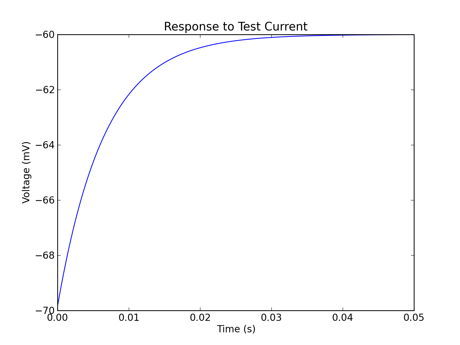
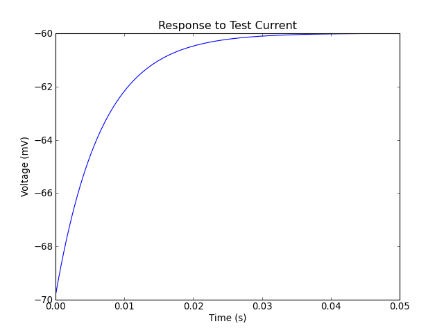
Typically, a user will estimate models from data using the fit_neuron.optimize.fit_gLIF.fit_neuron() function (which can be saved for future use using pickle) and hence does not need to know how to instanciate model instances from parameters only. The following plot and source code illustrates how a neuron can be loaded directly from parameter arrays. The meaning of the parameters is explained in Subthreshold Fitting Procedure Overview and Threshold Fitting Procedure Overview.
(Source code, png, hires.png, pdf)
Running a Test Script
To run a test script which estimates a model from data, execute the following at the command line:
python -m fit_neuron.tests.test
The contents of this script can be viewed at fit_neuron.tests.test and document much of this package’s functionality. The script will estimate the parameters for a neuron, save the parameters in a JSON file, save a model instance with pickle, plots and saves simulation figures, and plots and saves evaluation figures.
Note
By default, fit_neuron.tests.test.run_single_test() will save the output figures and data to a new directory test_output_figures located in the current directory.
Some Simulation Figures
Fitting results for neuron_1:
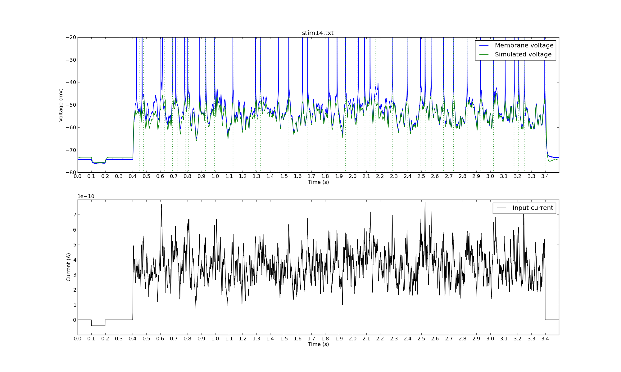
Another Monte Carlo simulation:
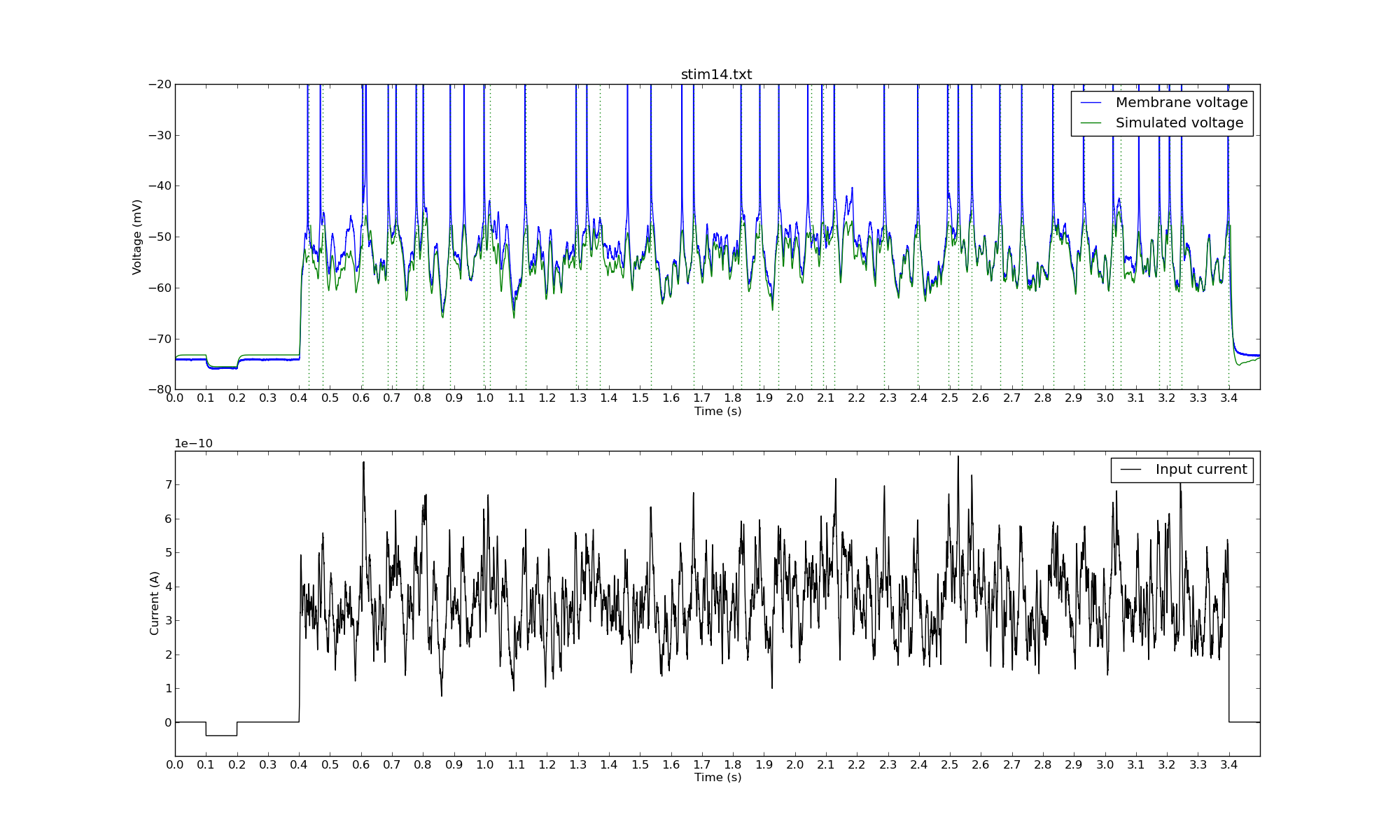
Note
The green dotted lines represent the times when the model neuron spiked.
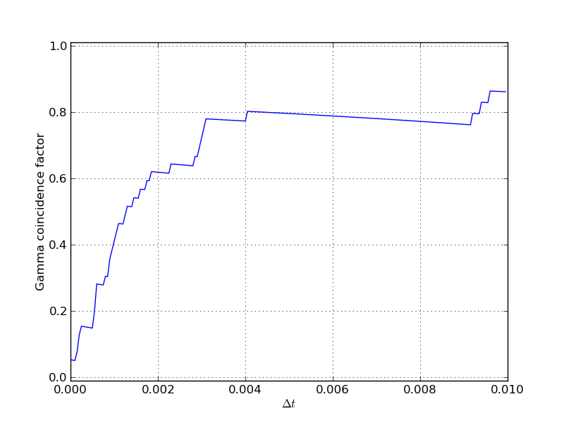
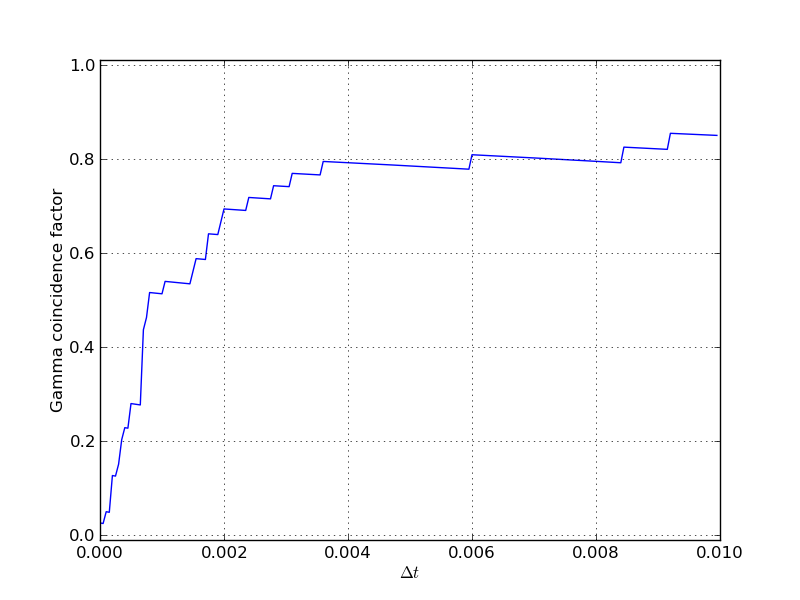
Some Statistics Figures
Here are some figures showing values of the Gamma coincidence factor
for different values of  .
.
Fitting results for neuron_1:
Another Monte Carlo simulation:
Here are some figures showing values of the Schreiber similarity measure
for different values of the bandwidth of the Gaussian kernel  .
.
Fitting results for neuron_1:

Another Monte Carlo simulation:
