A Guide to the Optimize Package ¶

Contents

A Guide to the Optimize Package

Overview ¶

The optimize package supports parameter estimation of stochastic generalized integrate and fire (gLIF) neurons from patch clamp data. In this document, we shall describe the following:

Model equations.

Object oriented implementation.

Optimization routines.

Model Summary ¶

The neurons estimated by the optimize packages consist of two components:

Subthreshold dynamics, which capture the dynamics of the membrane potential, its dependence on the input current, and its dependence on spike times. The subthreshold dynamics are implemented by fit_neuron.optimize.subthreshold.Voltage.
Threshold dynamics, which predicts the probability of a spike occuring depending on the current voltage and the past history of the neuron. The threshold dynamics are implemented by fit_neuron.optimize.threshold.StochasticThresh.

Subthreshold Equations ¶

The following difference equation defines the subthreshold model:

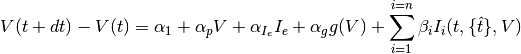
$V(t + dt) - V(t) = \alpha_1 + \alpha_p V + \alpha_{I_e} I_e + \alpha_g g(V) + \sum_{i=1}^{i=n} \beta_i I_i(t,\{\hat{t}\},V)$

where

$t$ is the current time
$dt$ is the time step, typically corresponding to the time step in the recorded patch clamp data
$\{\hat{t}\}$ is the set of previous spike times
The $I_i$ are the spike triggered currents or spike induced currents which depend only on the spiking history of the neuron, and optionally on the current value of the voltage $V$ .
The function $g(V)$ is a voltage nonlinearity function that allows the model to have an upward spike initiation. Commonly used voltage nonlinearities are the quadratic and exponential functions.

See fit_neuron.optimize.threshold.StochasticThresh for the implemenation of this difference equation.

Whenever a spike occurs (as determined by the threshold equations), the state of the neuron is updated as follows:

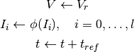
$V \gets V_r I_i \gets \phi(I_i), \quad i = 0,\hdots, l t \gets t + t_{ref}$

where

$V_r$ is the reset voltage.
$t_{ref}$ is the refractory period of the neuron.
$\phi$ is an optional update rule.

This update rule is implemented for general cases of spike induced currents by fit_neuron.optimize.subthreshold.Voltage.spike().

The Optimize package allows two variations of spike triggered currents.

Gerstner Adaptation Currents ¶

In [MS2011] the spike triggered currents take the form of a sum of step functions. This sum can be written as:

$I_i(t,\{\hat{t}\}) = \sum_{\hat{t} \in \{\hat{t}\}} I_{[0,a_{i} ]} (t - \hat{t})$

where the indicator functions $I_{[0,a_{i} ]}$ are defined as follows:

$I_{[0,a_{i}]}(x) = \begin{cases} 0, & \text{otherwise} \\ 1, & \text{if}\ x \in [0,a_{i}] \end{cases}$

By looking at the difference equation for the voltage, one sees that the parameter vector ${ \bf \beta } = [\beta_0,\hdots,\beta_n]^{\top}$ defines the shape of the spike triggered currents, and the $\{a_i\}$ parameters define the intervals during which the shape is constant.

In this case, the update rule simply appends the current spike to the spiking history $\{\hat{t}\}$ :

$\{\hat{t}\} \gets \{\hat{t}\} \cup t$

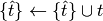
The Gerstner adaptation currents are implemented in fit_neuron.optimize.sic_lib.StepSic.

Note

The equations are written here in a form that matches the implemenation. The equations are written differently in [MS2011] but are perfectly equivalent up to a linear transformation of the parameter vector $\beta$ .

Mihalas-Niebur Adaptation Currents ¶

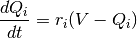
An alternative form of spike triggered currents is used in [MN2009] and consists of exponentially decaying currents with an additive reset. The equations are as follows:

$\frac{dI_i}{dt} = -k_i I_i$

and the reset equation, applied whenever the neuron spikes, is:

$\phi(I_i) = I_i + 1$

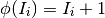
The Mihalas-Niebur adaptation currents are implemented in fit_neuron.optimize.sic_lib.ExpDecay_sic.

Object Oriented Implementation ¶

When calling the optimization routine fit_neuron.optimize.fit_gLIF.fit_neuron(), the user has the ability to specify any spike induced object he/she would like, as long as the user defines the class of the spike triggered current to inherit from the following abstract class: fit_neuron.optimize.sic_lib.SicBase.

Threshold Equations ¶

The stochastic neuron has the following hazard rate:

$h(t,V) = \exp \left( c_0 + c_1 V + \sum_{\hat{t} \in \{\hat{t}\}} \sum_{i=1}^{i=m} d_i I_{[0,b_i]} (t-\hat{t}) + \sum_{j=1}^{j=l} e_j Q_j(t) \right)$

where the $I_[0,b_i]$ parameters are the indicator variables (see above), and the $Q_j$ parameters are probability currents which shall be referred to as voltage chasing currents. These currents give the stochastic spike emission process a component that adapts to the history of the voltage. The equations used for the voltage chasing currents are:

$\frac{dQ_i}{dt} = r_i (V - Q_i)$

When the neuron spikes, the voltage chasing currents are set to the reset potential:

$Q_i \gets V_r$

The hazard rate is computed at each time step and compared to a uniformly distributed random number to determine whether the neuron spikes here. This computation is performed by fit_neuron.optimize.threshold.StochasticThresh.update_X_arr().

Fitting Procedure Overview ¶

The parameter estimation algorithm provided by the fit_neuron.optimize.fit_gLIF() function proceeds as follows:

Extract spikes and spike shapes from the raw data.
Take the voltage traces with the spike shapes removed, and estimate the subthreshold parameters by linear regression of the derivative of the voltage.
Simulate the model neuron using the same inputs as the raw data, and force the spikes to happen at the times the biological neuron was observed to spike. This will produce simulated voltage traces.
Fit the threshold parameters such that these parameters maximize the log likelihood of the obseved spike trains being emitted by the simulated voltage traces.

Subthreshold Fitting Procedure Overview ¶

The subthreshold parameters are obtained via linear regression to the observed voltage differences.

The equation that is solved is the following:

$\min_{b} \|Xb - Y\|^2$

where

$X = \begin{bmatrix} V(0) & 1 & I_e(0) & g(V) & I_0(0) & \hdots & I_n(0) \\ V(1) & 1 & I_e(1) & g(V) & I_0(1) & \hdots & I_n(1) \\ \vdots & \vdots & \vdots & \vdots &\vdots & \vdots & \vdots \end{bmatrix}$

and

$Y = \begin{bmatrix} V(1) - V(0) \\ V(2) - V(1) \\ \vdots \end{bmatrix}$

The value of $b$ that minimizes this expression is the parameter vector chosen for the subthreshold object fit_neuron.optimize.subthreshold.Voltage.

Note

The values of $V$ used above represent the values in the recorded voltage traces. The values of the spike induced currents $I_i(t)$ are computed based on the recorded voltage values and the recorded spike times. Hence the estimation process resembles maximum likelihood.

Note

If no voltage nonlinearity is provided, or if it is set to None, the parameter vector will still correspond to the $b$ vector above but with the voltage nonlinearity skipped.

Threshold Fitting Procedure Overview ¶

The threshold parameters are obtained via max likelihood of the observed spike train. Following along the lines of [MS2011] we may re-write the threshold equation in Threshold Equations as follows:

$h(t) = \exp \left({\bf w}_t^{\top} {\bf X}_t (t) \right)$

where

${\bf X}_t (t) = [1,V(t),I_1(t),\hdots,I_m(t),Q_1(t),\hdots,Q_l(t)]^{\top}.$

as computed by fit_neuron.optimize.threshold.StochasticThresh.update_X_arr().

The probability of there being a spike in a time increment $dt$ is

$p(t) = 1 - \exp \left(-h(t) dt \right)$

The probability of observing spikes at indices in the spiking set $S$ , and no spikes at the indices in the complement of this set $S^c$ , is:

$p(S) = \prod_{i \in S} p(t_i) \prod_{j \in S^c} (1 - p(t_j))$

Taking logs of both sides, we obtain

$L({\bf w}_t) = \sum_{i \in S} \log (p(t_i)) + \sum_{j \in S^c} \log(1 - p(t_j))$

which may be approximated up to a constant as:

$L({\bf w}_t) = \sum_{i \in S} {\bf w}_t^{\top} {\bf X}_t(t_i) - \sum_{j \in S^c} \exp \left({\bf w}_t^{\top} {\bf X}_t(t_j) \right)$

The $k$ ‘th elements of the gradient of this function w.r.t. ${\bf w}_t$ are:

$[\nabla L({\bf w}_t)]_k = \sum_{i \in S} [{\bf X}_t(t_i)]_k - \sum_{j \in S^c} [{\bf X}_t(t_j)]_k \exp \left({\bf w}_t^{\top} {\bf X}_t(t_j) \right)$

The $(l,m)$ elements of the Hessian matrix are:

$[H({\bf w}_t)]_{l,m} = - \sum_{j \in S^c} [{\bf X}_t(t_j)]_l [{\bf X}_t(t_j)]_m \exp \left({\bf w}_t^{\top} {\bf X}_t(t_j) \right)$

It is trivially seen that the Hessian matrix is negative definite. Hence the negative log likelihood is a convex function of the parameters and convex optimization techniques are applicable here. We use a Newton algorithm to update the values of the parameters:

${\bf w}_t^{\text{new}} = {\bf w}_t^{\text{old}} - H^{-1}({\bf w}_t) \nabla L({\bf w}_t)$

The most computationally expensive step in this process is the computation of the gradients and hessians, which must be done at every step. Significant speedups can be achieved by distributing the computations of the gradients and the hessians to multiple processors. This is done in fit_neuron.optimize.threshold.par_calc_log_like_update().

References ¶

[RB2005]

Brette, Romain, and Wulfram Gerstner. “Adaptive exponential integrate-and-fire model as an effective description of neuronal activity.” Journal of neurophysiology 94.5 (2005): 3637-3642.

[MN2009]

Mihalas, Stefan, and Ernst Niebur. “A generalized linear integrate-and-fire neural model produces diverse spiking behaviors.” Neural computation 21.3 (2009): 704-718.

[MS2011]

(1, 2, 3) Mensi, Skander, et al. “Parameter extraction and classification of three cortical neuron types reveals two distinct adaptation mechanisms.” Journal of neurophysiology 107.6 (2012): 1756-1775.

A Guide to the Optimize Package ¶

Overview ¶

Model Summary ¶

Subthreshold Equations ¶

Gerstner Adaptation Currents ¶

Mihalas-Niebur Adaptation Currents ¶

Object Oriented Implementation ¶

Threshold Equations ¶

Fitting Procedure Overview ¶

Subthreshold Fitting Procedure Overview ¶

Threshold Fitting Procedure Overview ¶

References ¶

Table Of Contents

Previous topic

This Page

Navigation

Previous topic

This Page

Quick search

Navigation