Geographic Networks

This tutorial was developed for the course Introduction to Digital & Computational Methods in the Humanities (HPS), created and taught by Julia Damerow and Erick Peirson.

Many bibliographic datasets include institutional affiliations for authors. Using geocoding services, such as the Google Geocoding API, we can convert institution names and addresses into geographic coordinates that can be plotted on a map. Tethne provides geocoding services in the services.geocode module.

In this tutorial, we will use the Google Geocoding service to obtain geographic coordinates for authors in a coauthorship network (see Coauthorship Networks) and its derivative, the institutions network (see networks.authors.institutions()). We will then plot those geo-coded networks in Gephi using the Geo Layout plugin, and overlay them on a 3D map of the globe in Google Earth.

The examples in this tutorial were generated using records for the journal Ecology from 2001-2013. See Getting Bibliographic Data.

Requirements

The Python package geopy must be installed and in your Python path. You should be able to install it using:

$ pip install geopy

Are your data suitable?

Not all bibliographic data is amenable to geocoding. When parsing data from the Web of Science, Tethne looks for author institutional affiliations in the C1 field. For example:

C1 [Keung, Jacky] Hong Kong Polytech Univ, Dept Comp, Kowloon, Hong Kong, Peoples R China.
   [Kocaguneli, Ekrem; Menzies, Tim] W Virginia Univ, Lane Dept Comp Sci & Elect Engn, Morgantown, WV 26505 USA.

Visually inspect your Web of Science data before proceeding. If most of your data lack the C1 field, then attempting to geocode a coauthorship network based on these data won’t be particularly fruitful. Try downloading a dataset that contains more recently-published records.

Since the Web of Science does not use controlled sub-fields for institution addresses, Tethne pays attention only to the first and last parts of each affiliation field. From Tethne’s perspective, then, the mapping between authors and institutions shown above becomes:

Author	Institution
KEUNG J	HONG KONG POLYTECH UNIV, PEOPLES R CHINA
KOCAGUNELI E	W VIRGINIA UNIV, WV 26505 USA
MENZIES T	W VIRGINIA UNIV, WV 26505 USA

When attempting to retrieve geographic information for these institutions, Tethne first attempts to retrieve a location for the institution itself, e.g. by passing HONG KONG POLYTECH UNIV, PEOPLES R CHINA to the geocoding service. If this does not yield a result, Tethne tries passing the last field only, e.g. PEOPLES R CHINA. Note that for most U.S. addresses, the state and zip code are included in the last field, e.g. WV 26505 USA. The method that successfully yielded a geographic result determines the precision field, discussed below.

Coauthorship network with geocoding

The networks.authors.coauthors() method accepts a boolean keyword argument called geocode. If geocode is True, Tethne will attempt to generate geographic coordinates for each node in the coauthorship network based on each authors’ institutional affiliation.

Follow the instructions in Coauthorship Networks to generate a coauthorship network. For the purpose of this tutorial, we will not generate a sliced/dynamic network. Command-line and Python users can skip the slice step; TethneGUI users should use the Ignore DataCollection slicing option. Also:

Command-line

• Skip the slice step.
• At the graph step, include the --merged and --geocode flags. For example:

$ python ~/Downloads/tethne-python/tethne -I fundata01 -O ~/results --graph \
> -N author -T coauthors --edge-attr=ayjid,date,jtitle --geocode --merged

TethneGUI

• Skip the Slice step.
• At the Graph step, check the Geocode option.

Python

Include the keyword argument geocode=True when calling networks.authors.coauthors(). For example:

>>> import tethne.networks as nt
>>> coauthors = nt.authors.coauthors(papers, threshold=2, geocode=True)

Export to GraphML

In order to visualize our geographic network in Gephi, we will export it to GraphML. See the section Write the Graph to GraphML in the Coauthorship Networks tutorial.

If everything went as planned, your GraphML nodes should contain three additional attributes: latitude, longitude, and precision. By default, networks.authors.coauthors() also includes the institution attribute. For example:

<node id="STEINGER T">
     <data key="latitude">52.132633</data>
     <data key="institution">UNIV WAGENINGEN &amp; RES CTR, NETHERLANDS</data>
     <data key="longitude">5.291266</data>
     <data key="precision">country</data>
</node>

Attribute	Description
latitude	Latitude on the Earth, in +/- degrees from the equator.
longitude	Longitude on the Earth, in +/- degrees from the Prime Meridian.
institution	The author’s institutional affiliation.
precision	The search pattern that yielded geographic data. If the geocoding service recognized the full institution address, then this will be institution. If only the last field was recognized, then this will be country.

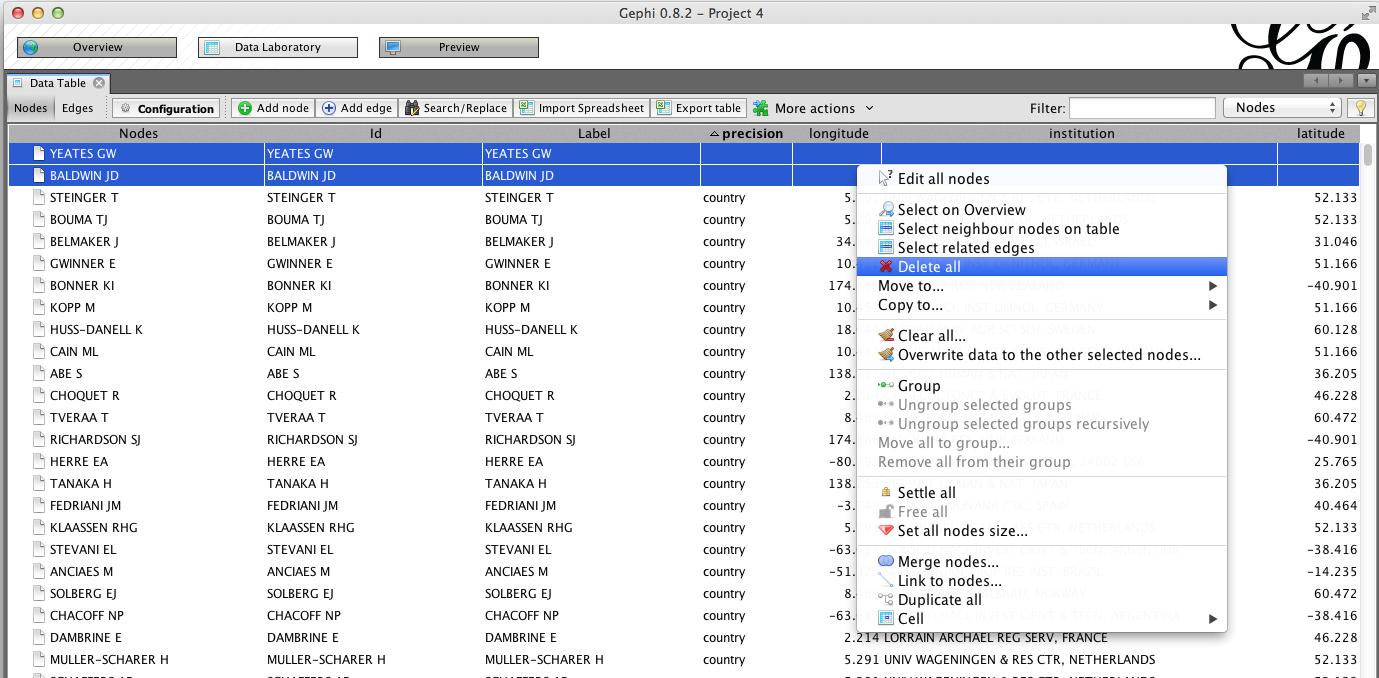
You may wish to remove nodes that do not contain geographic locations.

1. Click the label of the precision column to sort by precision; this should bring nodes without locations to the top of the list.
2. Select the nodes that do not have data in the location fields.
3. Right-click, and click Delete all.

Geo Layout in Gephi

Import your GraphML file as described in the section Inter-institutional Collaboration in Gephi in the Coauthorship Networks tutorial.

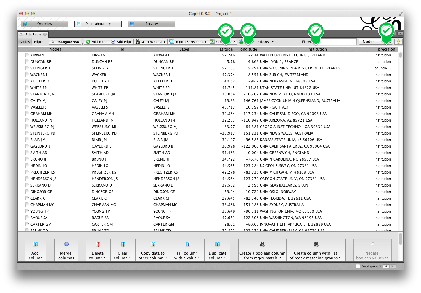
In the Data Laboratory tab, you should see columns for the four attributes described above.

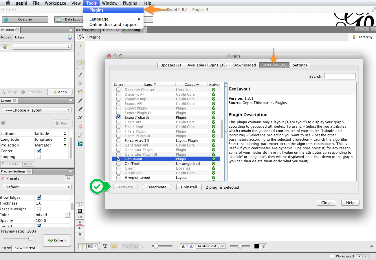
Make sure that both the GeoLayout and ExportToEarth plugins are installed.

1. In the File menu, go to Tools > Plugins. A new window called Plugins should appear.
2. Click on the Installed tab, and scroll through the list to find GeoLayout and ExportToEarth.
3. If those plugins are not installed, click the Available Plugins tab, select them from the list, and click the Install button.
4. Make sure that both plugs are active. In the Installed tab, select each plugin. If they are active, then the Activate button should be grayed out. If so, do nothing. If not, click Activate.
5. Click the Close button to return to the main Gephi interface.

Now you’re ready to run the GeoLayout.

• In the Layout area, select Geo Layout from the drop-down menu.
• Gephi should automatically detect and use the latitude and longitude attributes for your nodes.
• The default projection is Mercator; you can change this to suit your needs.
• Click the Run button.

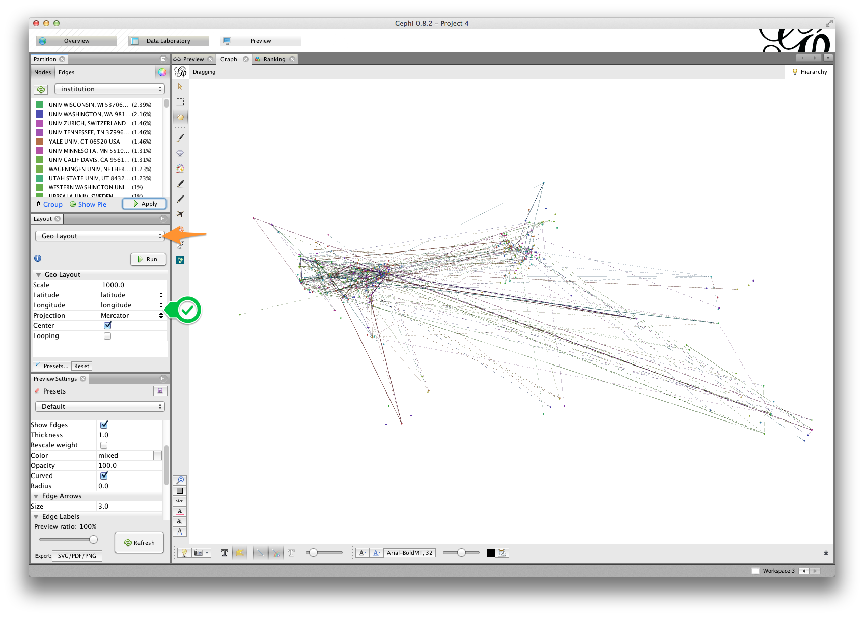
If your data are similar to the ones used in this tutorial, you should see something like the visualization shown in the figure above. The arrangement of the nodes is suggestive of some familiar national boundaries, especially the United States and western Europe.

In this example, we’ve also partitioned and colored nodes by institution. This will matter more when we plot this network in Google Earth, below.

Eigenvector Centrality

In this tutorial, we’ll introduce another measure of centrality popular in social network analysis.

Eigenvector Centrality is a measure of how well-connected a node is in a network. A node has high Eigenvector Centrality if it is connected to other highly-connected nodes. Google’s PageRank algorithm uses something like Eigenvector Centrality to find the most authoritative or important results for your search query: if a page receives in-links from other highly-authoritative webpages, it will appear higher in your search results. Unlike Degree Centrality, Eigenvector Centrality depends not merely on how many neighbors a node has, but also on how well-connected those neighbors are.

In social network analysis, a node with high Eigenvector Centrality might be a high-profile leader or public figure. In contrast to nodes with high Betweenness Centrality, however, nodes with high Eigenvector Centrality may not be strong “brokers”; they may not occupy structurally import positions in the network. For more details, see this blog post.

We’ll use Eigenvector Centrality to set the size of the nodes in our coauthorship network.

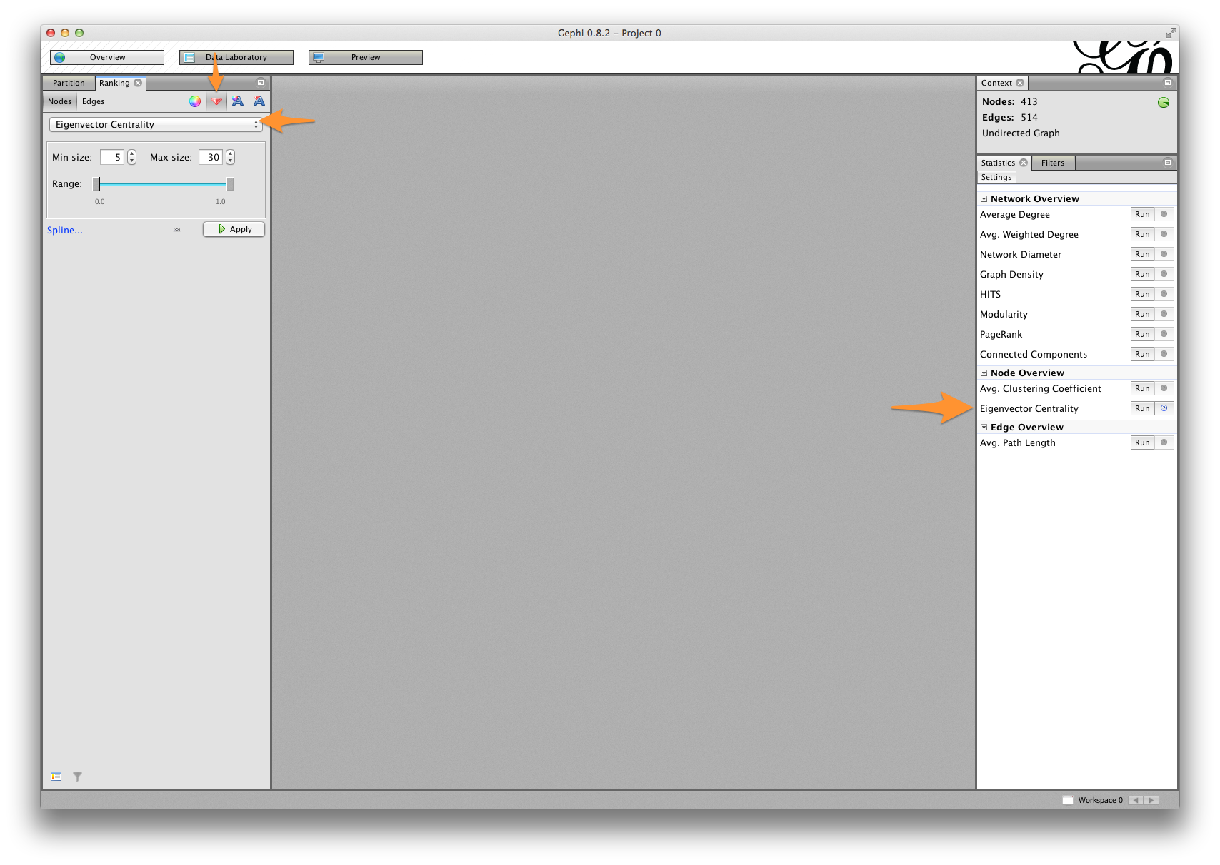
1. Go to the Overview tab.
2. In the Statistics window, find Eigenvector Centrality under Node Overview.
3. Click Run.

In the Data Laboratory tab, you should see a new column called Eigenvector Centrality.

To map node size to Eigenvector Centrality:

1. On the left-hand side of the Gephi workspace, find the Ranking window.
2. Select Eigenvector Centrality from the drop-down menu.
3. Click the red gem icon in the upper right.
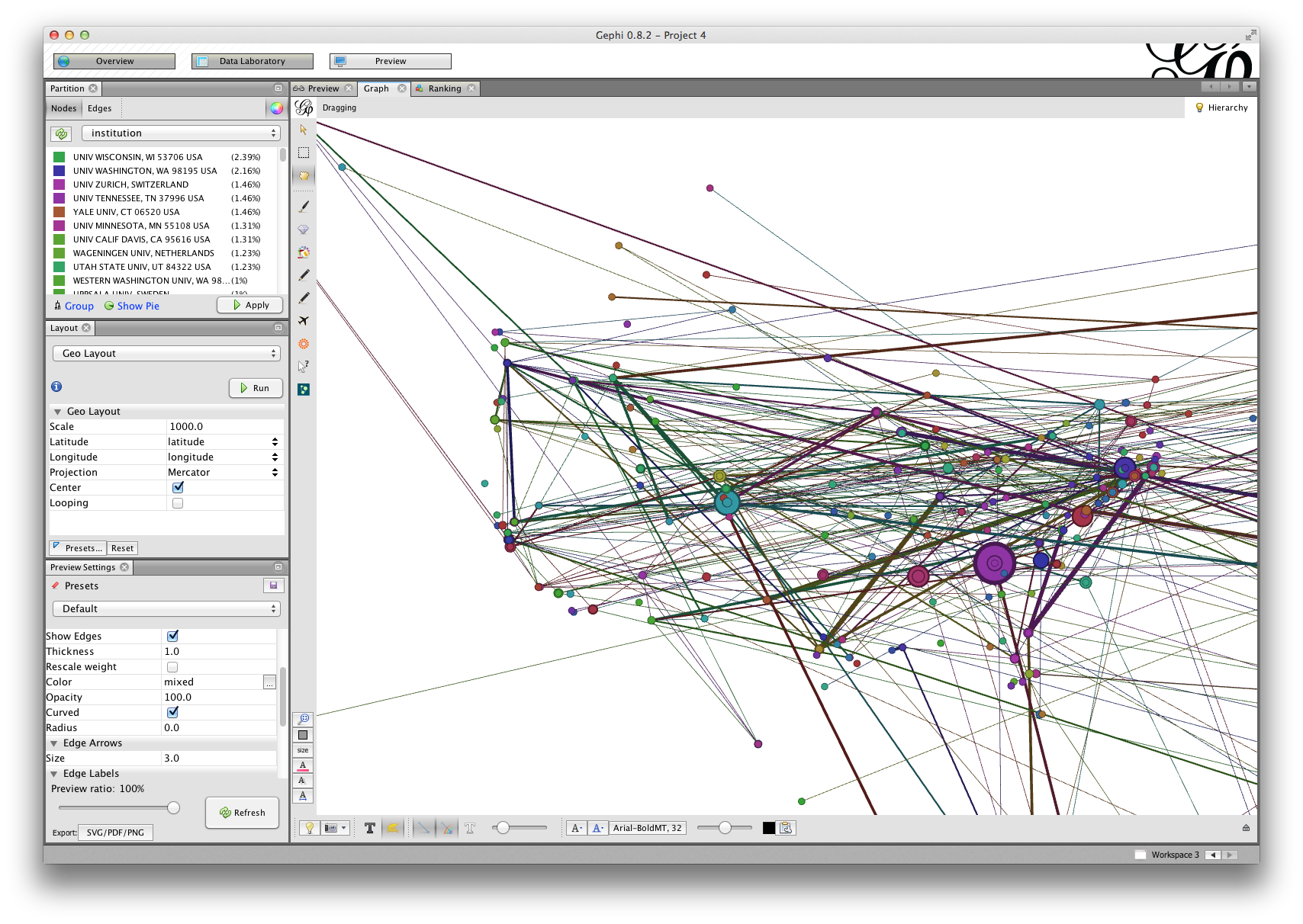
4. Specify a size range to define a linear function for node size vs centrality. You can define more complex functions by click on Spline... in the lower left of the Ranking window.
5. Click the Apply button, and return to Preview.

Zooming in on the United States, we can see that there are a few highly central individuals in the east and south, and one in Colorado. Note also that edge widths vary in size: Gephi automatically detected the weight attribute on edges between authors, which indicates how many papers a pair of authors published together.

Plotting geodata on a basemap

Unfortunately, Gephi does not provide any straightforward way to overlay networks on a map of the earth. One approach, which we will not address here, is to export your network view as a SVG (Scalable Vector Graphics) file, and then overlay that image on a basemap in a graphics editor (e.g. Photoshop or Gimp).

Another approach is to visualize your network in Google Earth. Google Earth reads a special kind of XML file called a Keyhole Markup Language (KML) files. The ExportToEarth plugin in Gephi allows you to save your geocoded network to a compressed KML, or KMZ, file.

Node size attribute

Before we export our network, we need to make one adjustment to our node attributes so that we can take our Eigenvector Centrality data along with us into Google Earth. When Gephi exports your network to KML, it looks for a size attribute on your nodes, which it uses to define a node size attribute in KML. Thus we need to copy our Centrality data into a size attribute before exporting to KML.

1. Go to the Data Laboratory.

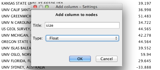
2. Create a new column by clicking on the Add column button in the lower left.

3. Name the column size, and select Float from the Type drop-down menu. Then click OK.

   

3. Click Copy data to other column and select Eigenvector Centrality.

   

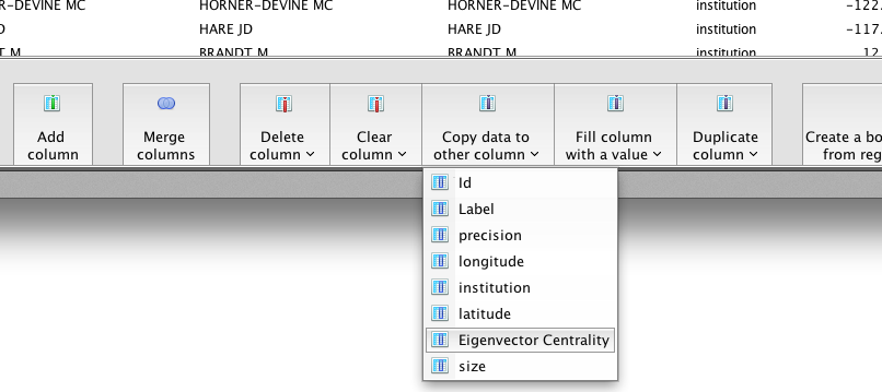
4. Select size from the drop-down menu, and click OK.

   

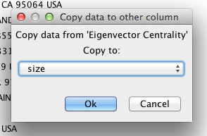
The Eigenvector Centrality and size columns should now contain precisely the same values.

Exporting KML (KMZ)

To export your network in KML...

1. Go to File > Export > Graph file....

   

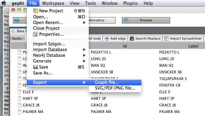
2. Select KMZ File (*.kmz) from the File Format drop-down menu.

   

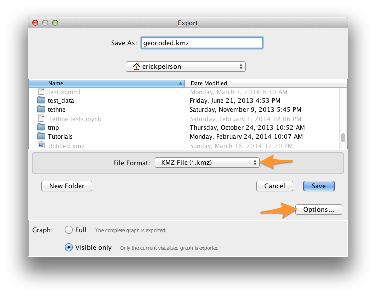
3. Give your file a name that you will remember; don’t remove the .kmz extension.

4. Click Options, and ensure that the checkbox next to size is checked, along with any other attributes that you’d like to take along.

   

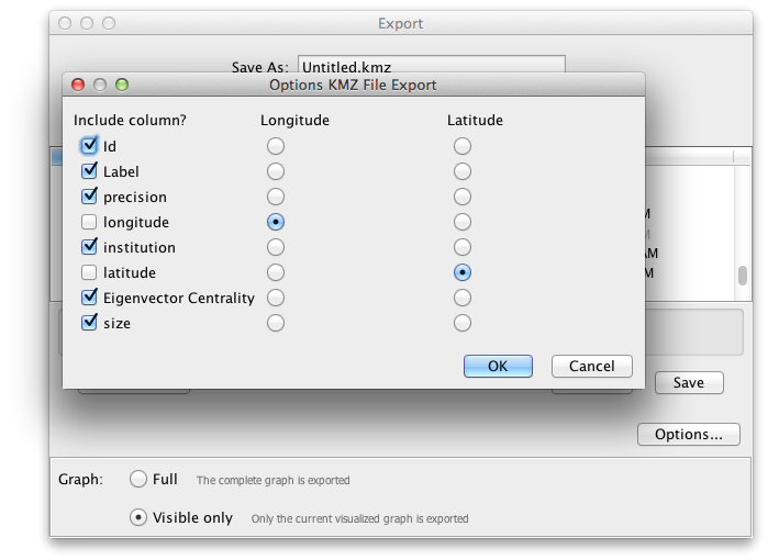
5. Click Save.

After a few moments, you should receive confirmation that your export is complete.

Visualization in Google Earth

Find your .kmz file in your computer’s filesystem. If Google Earth is installed properly, you should be able to simply double-click the file to open it. If that doesn’t work, start Google Earth, go to File > Open, and select your .kmz file.

If all goes well, you should see a bunch of nodes and lines criss-crossing a 3D image of the globe. For help navigating in Google Earth, see these tutorials.

If you zoom in on a particular region of the globe, you should notice a few things:

• Nodes come in different sizes, reflecting their Eigenvector Centrality as calculated in Gephi. Edges are also different sizes, reflecting their weight.

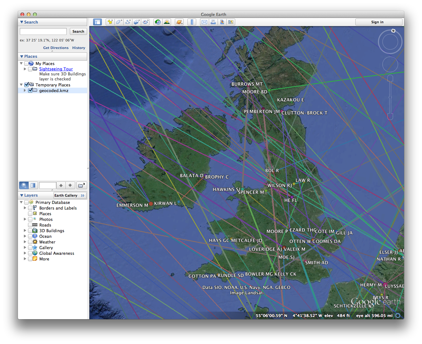
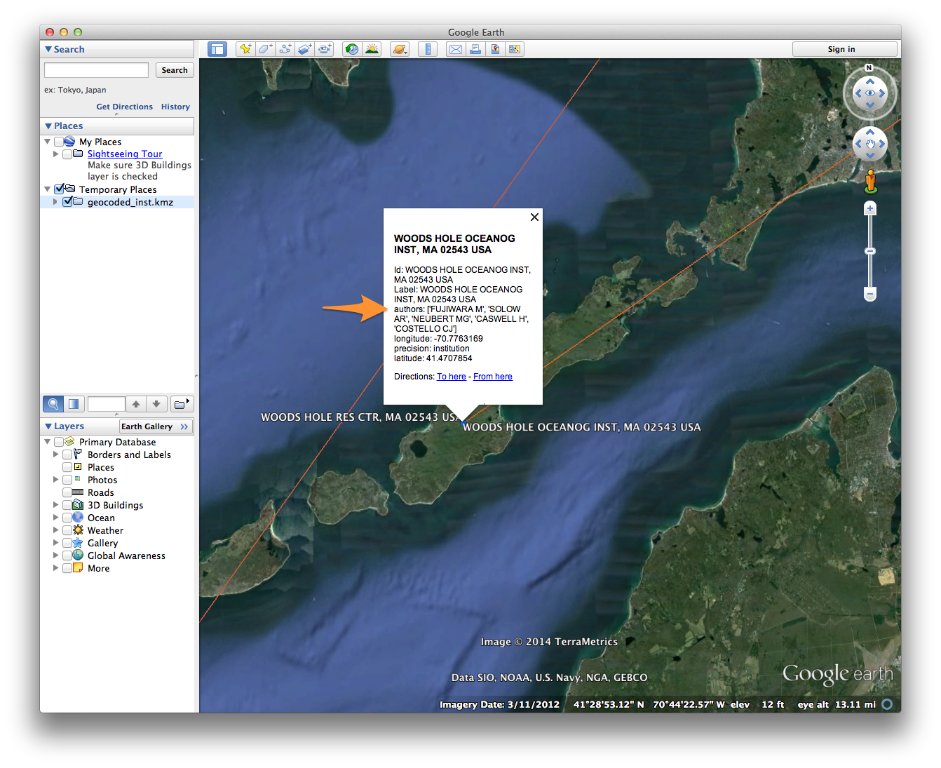
• Clicking on a node or edge reveals details about that element; e.g. the institution with which an author is affiliated.

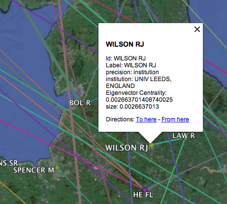
• In many cases, nodes will overlap. Clicking on a cluster of overlapping nodes will cause them to spread out, allowing you to select an individual node. Since node colors reflect the institutional partitioning that we did in Gephi, we can quickly see whether multiple institutions are represented at a particular locale.

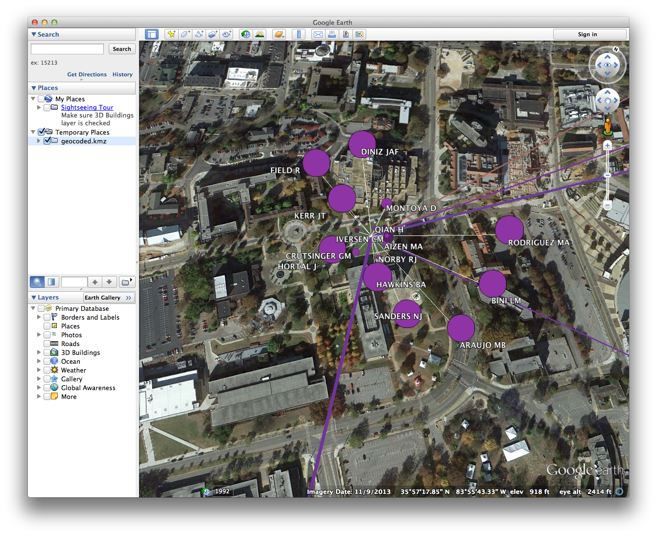
• Some nodes may not appear to be connected to any other nodes in the network. Since only individuals who coauthored papers with other researchers are included in the coauthorship network, those orphan nodes should represent cases in which an individual published only with other researchers at the same institution. Indeed, clicking on such a node should reveal at least two overlapping nodes at that location.

To export an image of your current view in Google Earth, click the Save Image icon in the menu bar. See Sharing Google Earth Screenshots. You can also record a tour!

Institutional Networks

Summary

In Coauthorship Networks we used Gephi’s partition tool to collapse our coauthorship network into an institutional network, in which the connections between institutional nodes represented coauthorship between individuals affiliated with those respective institutions. Unfortunately, the institutional nodes created by the partition procedure do not inherit the geographic attributes associated with the individuals in the original coauthorship network.

To deal with situations like this, Tethne has a network-building method called networks.authors.institutions() that produces geocoded institutional coauthorship networks. The size attribute on each node indicates the number of authors in the dataset associated with that institution, and the weight attribute on each edge indicates the total number of publications coauthored by individuals at a given pair of institutions.

Building an institutional network is almost precisely the same as building a coauthorship network (as above), with the following exceptions:

Command-line

At the graph step, use --graph-type=institutions.

TethneGUI

At the Build Graphs step, select institutions from the Graph type drop-down menu.

Python

Use networks.authors.institutions() instead of networks.authors.coauthors(). The call-signature is almost precisely the same. For example:

>>> inst = nt.authors.institutions(recent, threshold=2, geocode=True)

Visualization

Follow the same steps as those described above for visualizing your institutional network. This time you won’t need to create a size attribute (unless you wish to override it), as one is already set based on the number of authors affiliated with each institution.

When visualizing the institution network in Google Earth, clicking on a node reveals a list of all of the authors associated with that institution.