Bibliographic Coupling

Bibliographic coupling was first proposed as a method for detecting latent topical affinities among research publications by Myer M. Kessler at MIT in 1958. In 1972, J.C. Donohue suggested that bibliographic coupling could be used to the map “research fronts” in science, and this method, along with co-citation analysis and other citation-based clustering techniques, became a core methodology of the science-mapping craze of the 1970s. Bibliographic coupling is still employed in the context of both information-retrieval and science-studies.

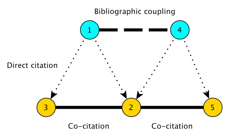
Two papers are bibliographically coupled if they both cite at least some of the same papers. The core assumption of bibliographic coupling analysis is that if two papers cite similar literatures, then they must be topically related in some way. That is, they are more likely to be related to each other than to papers with which they share no cited references.

This tutorial provides a walk-through for building bibliographic coupling networks from Web of Science citation data, using the command-line interface, the TethneGUI (developed for demonstration purposes only), and the Python API.

The section Cluster Detection introduces Cytoscape’s MCODE clustering app.

Before you begin, be sure to install the latest version of Tethne. Consult the Installation guide for details.

If you run into problems, don’t panic. Tethne is under active development, and there are certainly bugs to be found. Please report any problems on our GitHub issue tracker.

Getting Started

Before you start, you should choose an output folder where TethneGUI should store graphs and descriptions of your dataset.

You should also choose a dataset ID. This is a unique ID that Tethne will use to keep track of your data between workflow steps.

Initialize TethneGUI

When you first start TethneGUI, you should see a window like the one shown below. Click Select folder... to specify your output folder. A dataset ID should be automatically generated for you; you can change this if you wish.

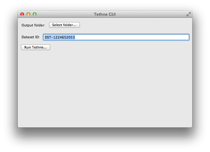
Once you’ve selected an output folder and a dataset ID, click the Run Tethne... button.

Reading WoS Data

You can read WoS data from one or multiple field-tagged data files.

Command-line

Use -I examplID to specify your dataset ID, and -O /Users/erickpeirson/exampleOutput to specify your output folder.

--data-format=WOS tells Tethne that your data are in the Web of Science field-tagged format.

$ tethne -I exampleID -O /Users/erickpeirson/exampleOutput --read-file \
--data-path=/Users/erickpeirson/Downloads/tests/savedrecs4.txt --data-format=WOS
----------------------------------------
        Workflow step: Read
----------------------------------------
Reading WOS data from file /Users/erickpeirson/Downloads/tests/savedrecs4.txt...done.
Read 500 papers in 2.67462515831 seconds. Accession: 0ff65dc3-b8f7-4bdc-a714-2d2a539f10a9.
Generating a new DataCollection...done.
Saving DataCollection to /tmp/exampleID_DataCollection.pickle...done.

TethneGUI

1. Select your WoS data file. If you have one data file, click the Select a File.... If you have multiple data files in their own folder, click Select a Folder....
2. Select the WOS file format.
3. Click the Read files button.

Depending on the size of your dataset, this may take a minute or two. When TethneGUI is done reading your data, you should see messages like those depicted in the image below.

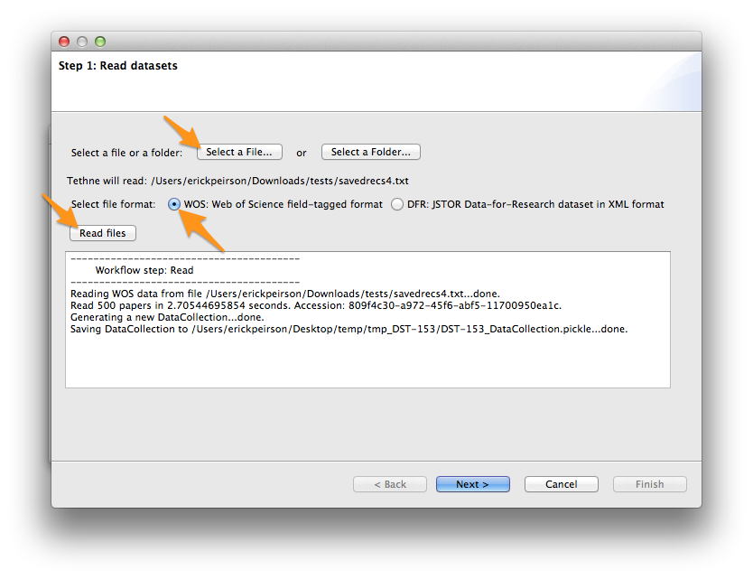
If your data are read successfully, click Next >.

Python

First import the tethne.readers module, then use the readers.wos.read() method to create a list of Paper instances. You can use readers.wos.from_dir() to import all of the WoS datafiles in a directory.

>>> # Parse data.
>>> import tethne.readers as rd
>>> papers = rd.wos.read("/Path/To/FirstDataSet.txt")

Then create a new DataCollection to organize your data.

>>> from tethne.data import DataCollection
>>> D = DataCollection(papers)

Slicing WoS Data

In this tutorial, we will first build a static bibliographic coupling network using all of the records in your WoS dataset. Then, if your dataset contains records from across a broad time-domain, you may also wish to view the evolution of your bibliographic coupling network over time by slicing your data using a sliding time-window. Since we can choose to merge our data slices in the graph step, we’ll go ahead and slice our data now.

The sliding time-window slice method is a bit different than the simple time-period slice method used in the Coauthorship Networks tutorial. Whereas time-period slicing divides data into subsets by sequential non-overlapping time periods, subsets generated by time-window slicing can overlap.

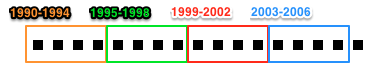
Time-period slicing, with a window-size of 4 years.

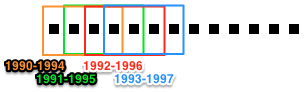
Time-window slicing, with a window-size of 4 years and a step-size of 1 year.

Command-line

$ tethne -I exampleID -O /Users/erickpeirson/exampleOutput --slice -S date \
> -M time_window --window-size=4
----------------------------------------
        Workflow step: Slice
----------------------------------------
Loading DataCollection from /tmp/exampleID_DataCollection.pickle...done.
Slicing DataCollection by date...done.
Saving slice distribution to /Users/erickpeirson/exampleOutput/exampleID_sliceDistribution.csv...done.
Saving sliced DataCollection to /tmp/exampleID_DataCollection_sliced.pickle...done.

TethneGUI

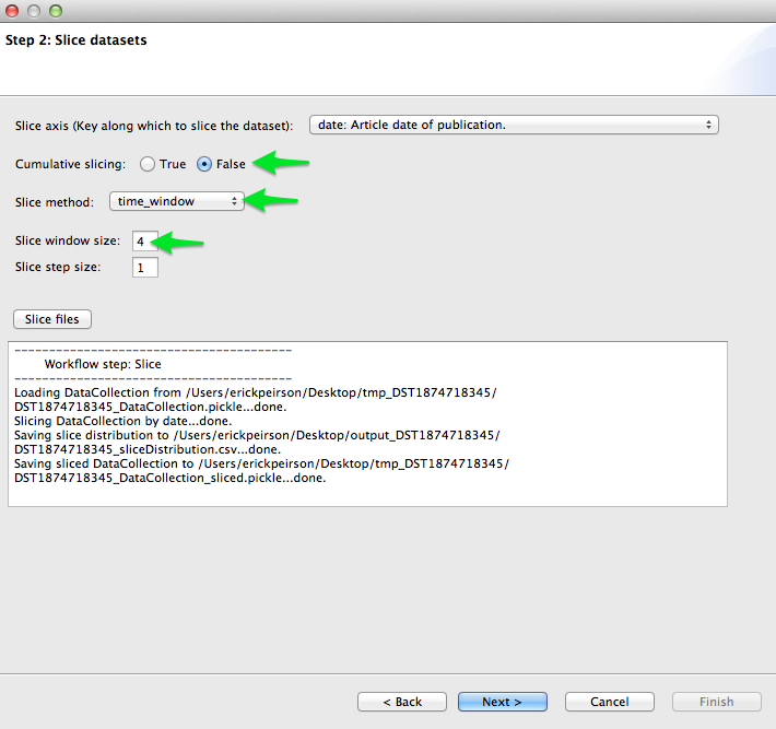
1. The slice axis should be set to date by default. If not, select it from the Slice axis drop-down menu.
2. Set Cumulative slicing to False.
3. Select time_window from the Slice method menu.
4. Set the Slice window size to 4.
5. Click Slice files.

After a few minutes, slicing should be complete; click Next >.

Python

Use the tethne.data.DataCollection.slice() method to slice your data.

>>> D.slice('date', 'time_window', window_size=4)

Building the Bibliographic Coupling Graph

For now, we’ll ignore data slicing and generate a single bibliographic coupling graph from the entire dataset using the merged option. Later on, we’ll come back and use the data slicing to look at how the network evolves over time.

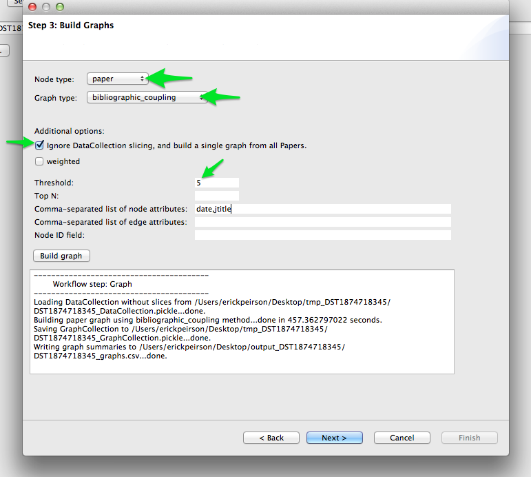
To generate a bibliographic coupling network, we will tell Tethne to use papers for nodes, and use the bibliographic_coupling graph type. For a complete list of graph types available in Tethne, see networks.

Generating an informative graph using bibliographic coupling will require some tuning. Depending on the criteria that you used to generate your bibliographic dataset, you may need to adjust the coupling threshold. Papers from a relatively narrow field have a high probability of sharing cited references, thus a threshold of 1 shared reference will result in a nearly complete graph that yields little information about the latent topical structure of that literature. If your dataset contains papers from quite disparate fields, however, you may wish to keep the threshold low.

Since papers vary widely in the total number of references that they cite, it may be desirable to use a normalized overlap value rather than an absolute one. If the weighted parameter is set to True, Tethne will use the normalized similarity metric s:

\[s = \frac{N_{i|j}}{\sqrt{ N_i N_j }}\]

If you choose to use absolute overlap (weighted is False), we suggest starting with a threshold of 5, and then adjusting it upward or downward to achieve optimal clustering. If you choose to use normalized overlap (weighted is True), then try starting with a threshold of 0.05.

We’ll also include some node attributes: date, jtitle (journal title), and atitle (article title).

Command-line

The value of the --node-attr argument should be a list of keys from the Paper class, separated by commas (no spaces).

$ tethne -I exampleID -O /Users/erickpeirson/exampleOutput --graph --merged \
> --node-type=paper --graph-type=bibliographic_coupling --threshold=0.05 --weighted \
> --node-attr=date,jtitle,atitle
----------------------------------------
        Workflow step: Graph
----------------------------------------
Loading DataCollection without slices from /tmp/exampleID_DataCollection.pickle...done.
Building author graph using coauthors method...done in 0.144234895706 seconds.
Saving GraphCollection to /tmp/exampleID_GraphCollection.pickle...done.
Writing graph summaries to /Users/erickpeirson/exampleOutput/exampleID_graphs.csv...done.

TethneGUI

Select author from the Node type menu, and coauthors from the Graph type menu. Check the Ignore DataCollection slicing option, then click Build graph.

Once the graph is built, click Next >. For now, we’ll skip the analysis step. Click Next > again to reach Step 5: Write graph(s).

Python

To generate a single graph from your DataCollection, call the coauthors() method directly from the networks.authors module.

Use the threshold and node_attribs keyword arguments to set the minimum coupling threshold and node attributes, respectively. node_attribs should be a list of string keys from Paper.

>>> import tethne.networks as nt
>>> bc_graph = nt.papers.bibliographic_coupling(D.papers(), threshold=5,
...                                            node_attribs=['date','jtitle','atitle'])

Write the Graph to GraphML

GraphML is a widely-used static network data format. We will write our network to GraphML for visualization in Cytoscape.

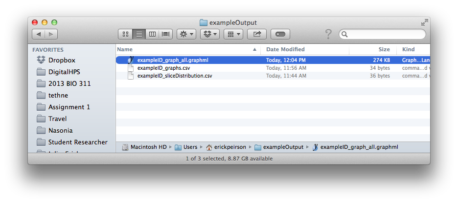
This step should generate a file in your output folder called [DATASET_ID]_graph_all.graphml.

Command-line

$ tethne -I exampleID -O /Users/erickpeirson/exampleOutput --write \
> --write-format graphml
----------------------------------------
        Workflow step: Write
----------------------------------------
Loading GraphCollection from /tmp/exampleID_GraphCollection.pickle...done.
Writing graphs to /Users/erickpeirson/exampleOutput with format graphml...done.

TethneGUI

Select graphml from the Output format for graph(s) menu, then click Write graph(s).

Python

Use the to_graphml() method in writers.collection to create a GraphML data file.

>>> import tethne.writers as wr
>>> wr.graph.to_graphml(bc_graph, "[OUTPUT_PATH]")

[OUTPUT_PATH] should be a path to the GraphML file that Tethne will create.

Visualizing the Merged Network

Cytoscape was developed in 2002, with funding from the National Instute of General Medical Sciences and the National Resource for Network Biology. The primary user base is the biomedical research community, especially systems biologists who study gene or protein interaction networks and pathways.

You can download Cytoscape 3 from url{http://www.cytoscape.org}. This tutorial assumes that you are using Cytoscape 3.1.

Import

In Cytoscape, import your network by selecting File > Import > Network > From file... and selecting the GraphML file generated by Tethne in your output directory.

Tethne includes the similarity of each pair of papers as an edge attribute. You can tell Cytoscape to take similarity into account when laying out your graph. To apply an edge-weighted layout, select Layout > Edge-weighted Spring Embedded > similarity.

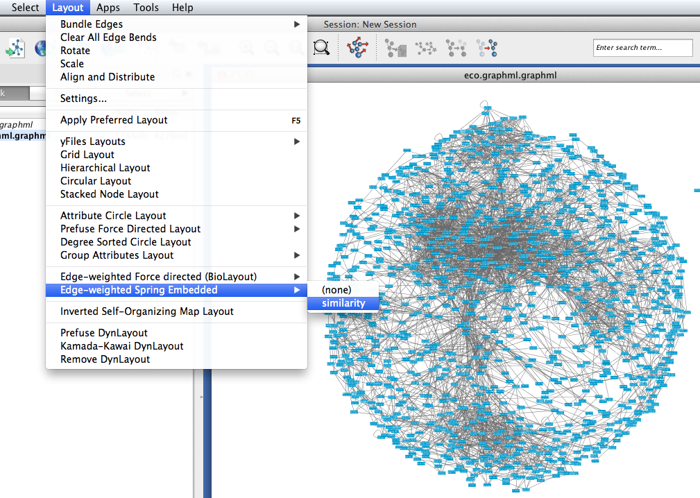
Your network may look like a giant hairball. If you can’t see much structure at all, you may wish to go back and rebuild the graph with a higher threshold. If your network is very sparse, you may wish to lower the threshold.

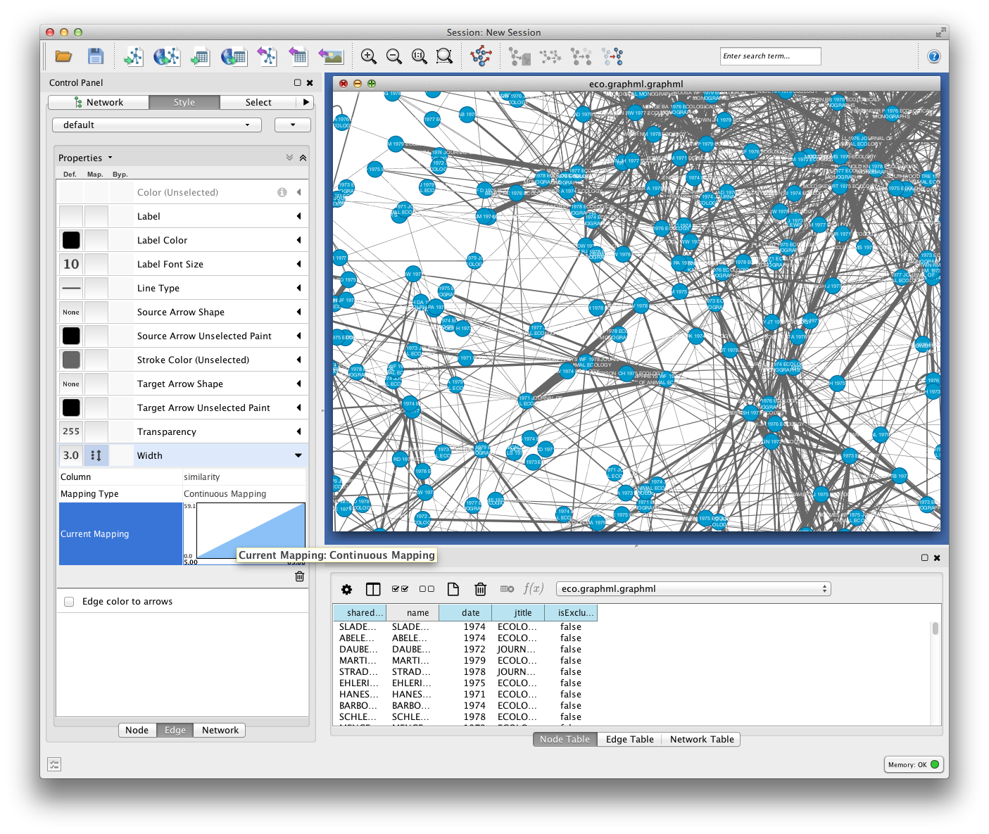
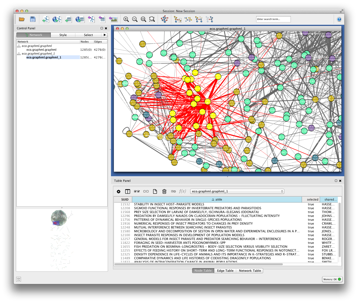
Set edge weight as a function of similarity to see which links are the strongest in your network.

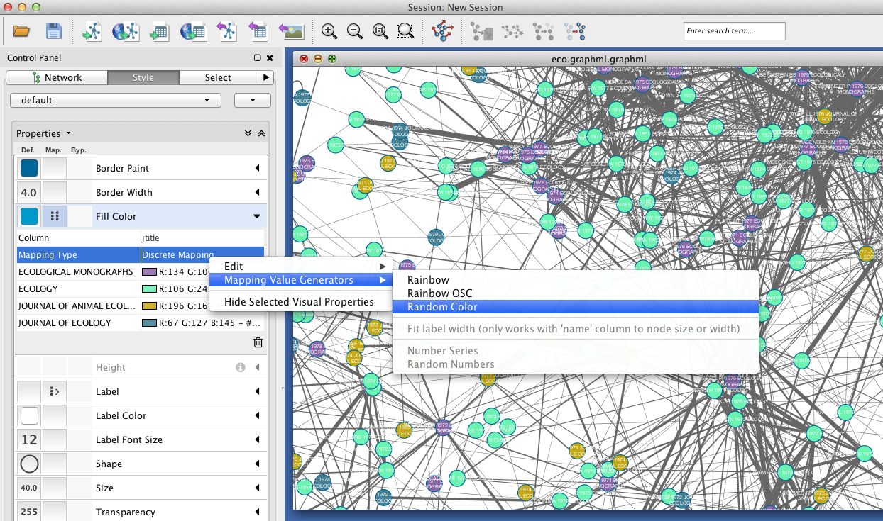
To get some idea of whether certain clusters in the network correspond to publication in the same journal, set node fill color as a discrete function of jtitle. You can automatically generate node fill colors by right-clicking on the visual mapping, and selecting Mapping Value Generators > Random Color.

Since you included the title of each paper (atitle) as a node attribute, you can get some idea of what makes a particular region of the network hang together by selecting some nodes and inspecting the Node Table in the Table Panel. In the example below, a quick visual inspection suggests that parasites figure heavily in the selected papers.

Cluster Detection

Especially if your network is very dense, it may be difficult to find salient clusters by visual inspection alone. Clustering algorithms provide a useful way to find groups of nodes that hang together in some way. Most clustering algorithms use an optimization function to find groups of nodes that are more densely connected among themselves than with the rest of the network.

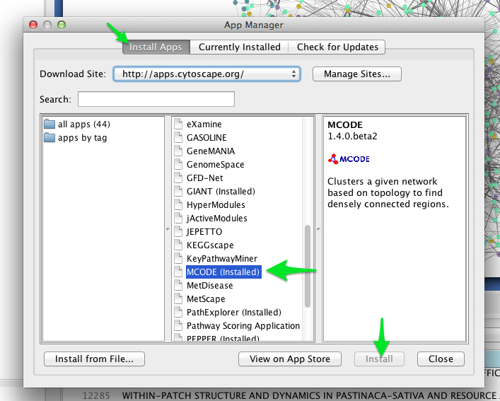
One such clustering algorithm in Cytoscape is provided by the MCODE app. To install the MCODE app:

1. Select Apps > App Manager from the main menu.
2. Click on the Install Apps tab, and find MCODE in the list of available apps.
3. Click the Install button.

MCODE should now appear in the Apps menu.

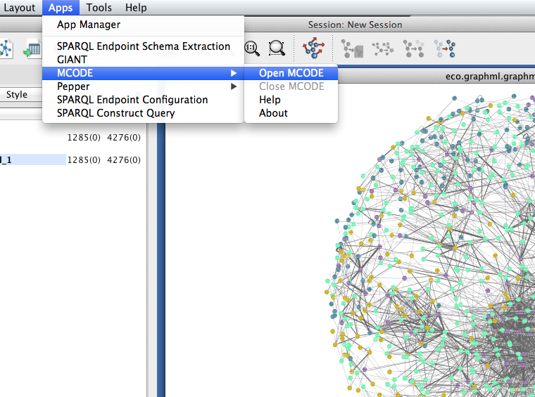
1. Select Apps > MCODE > Open MCODE. A new tab should appear in the Control Panel at left.
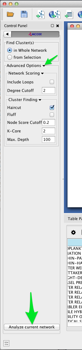
2. To adjust the parameters of the MCODE cluster-finding algorithm, expand the Advanced Options. MCODE works reasonable well with the default settings.
3. Click the Analyze current network button.

After a few moments, a new window should appear on the right side of the Cytoscape workspace. Click on a cluster in the Cluster Browser to select all of the nodes in that cluster. In some cases, MCODE will find clusters that are not at all obvious visually. This should give you an impression of the limitations of two-dimensional layouts for studying network structure, especially in very large, dense networks.

In the example below, MCODE has found a cluster of papers dealing with invertebrate predators in marine inter-tidal zones.

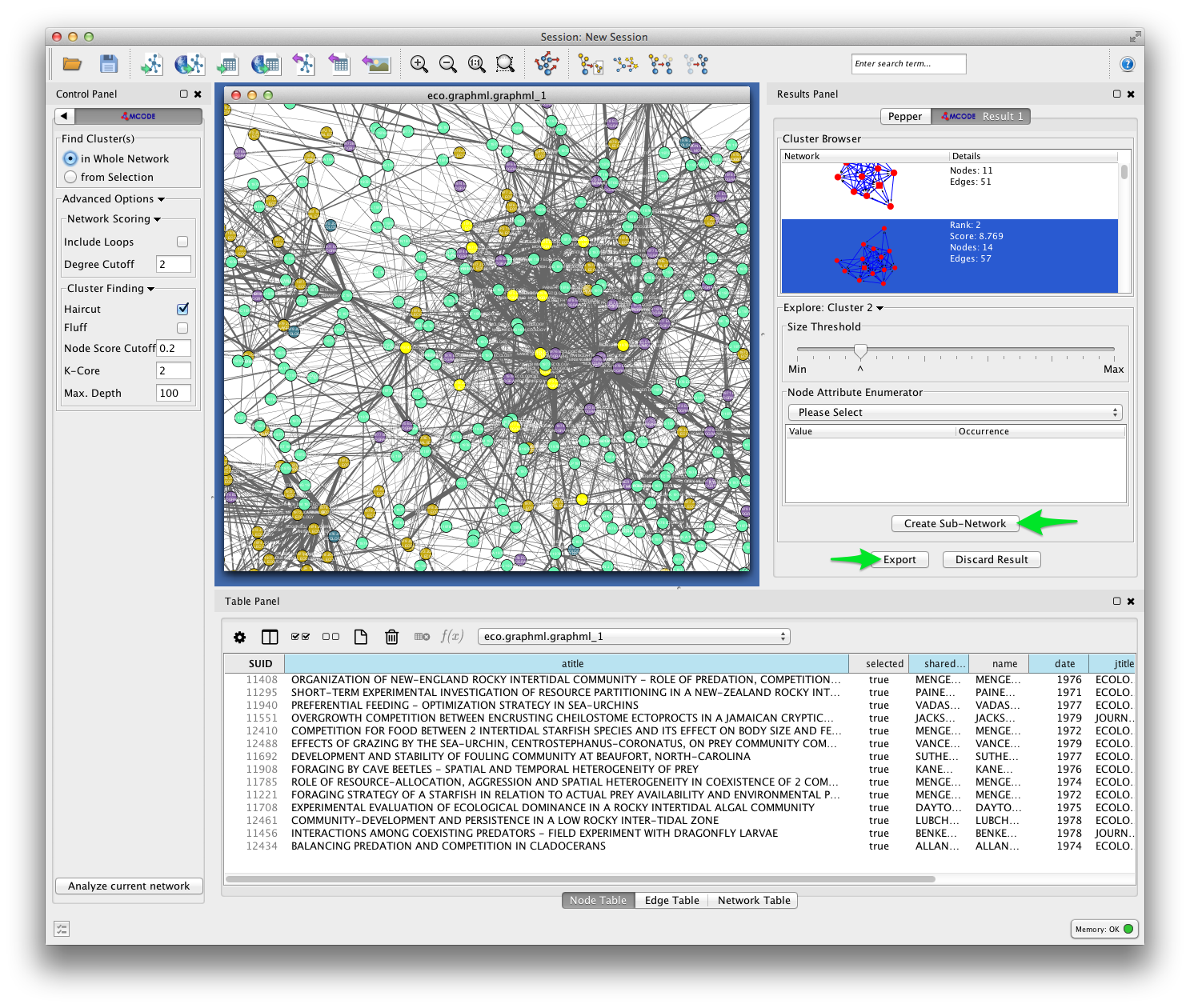
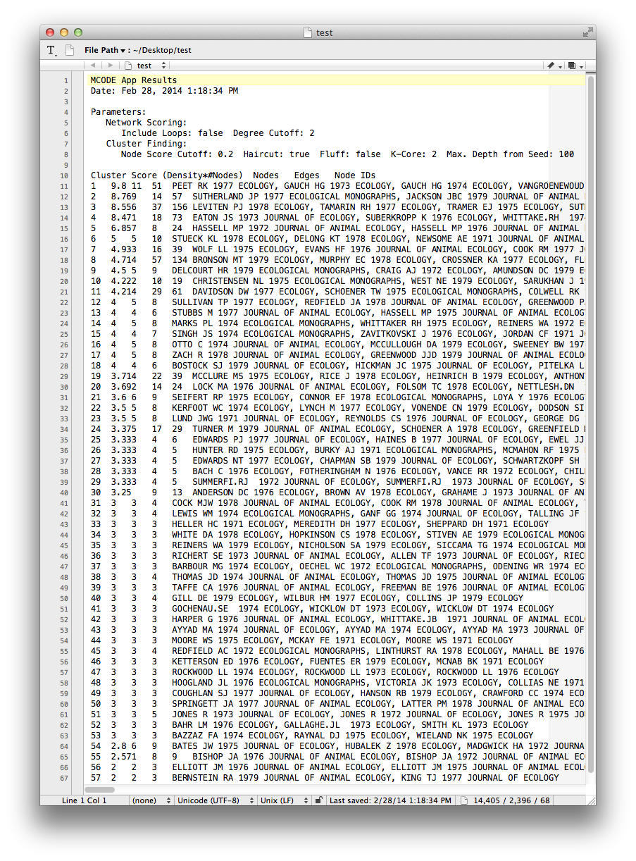
MCODE allows you to create a subnetwork from the selected cluster, or export your results. Exporting your results produces a table like the one shown below, listing each of the detected clusters and the papers the belong to them.

Future versions of Tethne will use this result to generate labels for each cluster based on the terms that uniquely characterize those groups of papers.

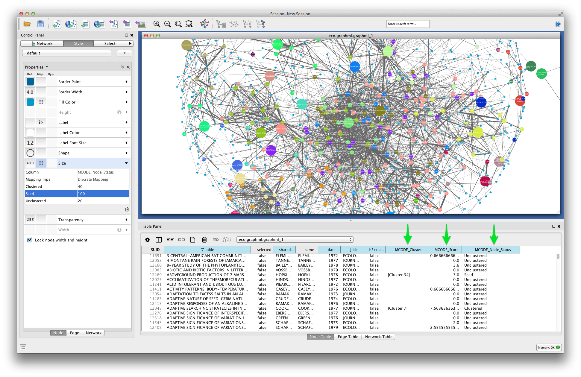
MCODE sets three node attributes:

• MCODE_Cluster contains the name of the cluster to which each node belongs.
• MCODE_Score indicates how strongly the neighbors around a node cluster together. This is similar to the Local clustering coefficient
• MCODE_Node_Status indicates whether a node is clustered, unclustered, or a seed node. Seed nodes are the reference nodes chosen by MCODE at the start of the cluster-detection process.

In the visualization below, node fill color is mapped to MCODE_Cluster. Node size is mapped to MCODE_Node_Status: unclustered nodes are small, seed nodes are large, and clustered nodes are intermediate in size.

Bibliographic Coupling over Time

If your dataset includes papers published over a long period of time, you may wish to analyze your bibliographic coupling graph as a dynamic network. This can give a visual impression of how fields and subfields evolve over time, in terms of whether they do or do not share cited references.

Command-line

Run the graph step again, but this time remove the --merged flag. This will create a separate graph from each of the data subsets created in the slice step.

$ tethne -I exampleID -O /Users/erickpeirson/exampleOutput --graph \
> --node-type=paper --graph-type=bibliographic_coupling --threshold=0.05 --weighted \
> --node-attr=date,jtitle,atitle
----------------------------------------
        Workflow step: Graph
----------------------------------------
Loading DataCollection with slices from /tmp/exampleID_DataCollection_sliced.pickle...done.
Using first slice in DataCollection: date.
Building author graph using coauthors method...done in 0.291323900223 seconds.
Saving GraphCollection to /tmp/exampleID_GraphCollection.pickle...done.
Writing graph summaries to /Users/erickpeirson/exampleOutput/exampleID_graphs.csv...done.

Re-run the write step. Use --write-format xgmml to select the dynamic XGMML export option.

$ tethne -I exampleID -O /Users/erickpeirson/exampleOutput --write --write-format xgmml
----------------------------------------
        Workflow step: Write
----------------------------------------
Loading GraphCollection from /tmp/exampleID_GraphCollection.pickle...done.
Writing graphs to /Users/erickpeirson/exampleOutput with format xgmml...done.

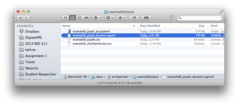
This should create a new file called [DATASET_ID]_graph_dynamic.xgmml in your output folder.

TethneGUI

Use the < Back button to return to Step 3: Build Graphs. Uncheck the Ignore DataCollection slicing option, and then click the Build graph button again. Then click Next >.

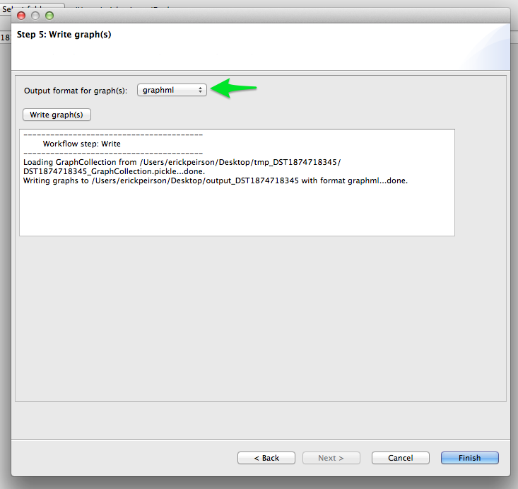
Skip the analyze step.

At the write step, select xgmml in the Output format menu, and click Write graph(s). This should create a new file called [DATASET_ID]_graph_dynamic.xgmml in your output folder.

Python

Use the paperCollectionBuilder to build a GraphCollection from your DataCollection.

>>> from tethne.builders import paperCollectionBuilder
>>> builder = paperCollectionBuilder(D)
>>> C = builder.build('date', 'bibliographic_coupling', threshold=5,
...                    node_attribs=['date','jtitle','atitle'])

Use the writers.collection.to_dxgmml() method to create dynamic XGMML.

>>> import tethne.writers as wr
>>> wr.collection.to_dxgmml(C, "[OUTPUT_PATH]")

[OUTPUT_PATH] should be a path to the XGMML file that Tethne will create.

Visualization

See Visualizing a dynamic network in Cytoscape for instructions about how to visualize your dynamic network in Cytoscape (the parts about attachment_probability don’t apply).