6. The `roots` module¶

New in version 0.4.

Here are some root-finding algorithm, such as ruffini()‘s method, quadratic() formula, cubic() formula, newton()‘s method, halley()‘s method, householder()‘s method, schroeder()‘s method, brent()‘s method, and bisection().

6.1. Simple algorithms and formulas¶

pypol.roots.ruffini(poly)¶

Returns the real integer roots (if there are any) of the polynomial basing on the right-hand side. If the polynomial has not the right-hand side, returns an empty list.

Examples

>>> p = poly1d([1, 5, 5, -5, -6])
>>> p
+ x^4 + 5x^3 + 5x^2 - 5x - 6
>>> ruffini(p)
[-1, 1]
>>> p(-1), p(1)
(0, 0)

and we can go on:

>>> p2, p3 = p / (x - 1), p / (x + 1)
>>> p2, p3
(+ x^3 + 6x^2 + 11x + 6, + x^3 + 4x^2 + x - 6)
>>> ruffini(p2), ruffini(p3)
([-1, -2, -3], [1])
>>> p2(-1), p2(-2), p2(-3)
(0, 0, 0)
>>> p3(1)
0
>>> p4, p5, p6 = p2 / (x - 1), p2 / (x - 2), p / (x - 3)
>>> p4, p5, p6
(+ x^2 + 7x + 18, + x^2 + 8x + 27, + x^3 + 8x^2 + 29x + 82)
>>> ruffini(p4), ruffini(p5), ruffini(p6)
([], [], [])

there are no more real roots, but if we try quadratic():

>>> quadratic(p4), quadratic(p5)
(((-3.5+2.3979157616563596j), (-3.5-2.3979157616563596j)), ((-4+3.3166247903553998j), (-4-3.3166247903553998j)))

New in version 0.3.

pypol.roots.quadratic(poly)¶

Finds the two roots of the polynomial poly solving the quadratic equation: $ax^2 + bx + c = 0$

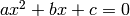
with the formula:: $\frac{-b\pm \sqrt{b^2 - 4ac}}{2a}$

Raises :	`AssertionError` if the polynomial’s degree is not 2.
Return type:	2 numbers (integer, float or complex) in a tuple

Examples

>>> p = poly1d([1, 0, -4])
>>> p
+ x^2 - 4
>>> quadratic(p)
(2.0, -2.0)
>>> p(2)
0
>>> p(-2)
0
>>> p = poly1d([2, 3, 1])
>>> p
+ 2x^2 + 3x + 1
>>> quadratic(p)
(-0.5, -1.0)
>>> p(-0.5)
0.0
>>> p(-1.0)
0.0

this functions can return complex numbers too:

>>> p = poly1d([-4, 5, -3])
>>> p
- 4x^2 + 5x - 3
>>> quadratic(p)
((0.625-0.59947894041408989j), (0.625+0.59947894041408989j))

but the precision is lower:

>>> p = poly1d([-4, 5, -3])
>>> p
- 4x^2 + 5x - 3
>>> quadratic(p)
((0.625-0.59947894041408989j), (0.625+0.59947894041408989j))
>>> r1 = (0.625-0.59947894041408989j)
>>> p(r1)
(-4.4408920985006262e-16+0j)
>>> r2 = (0.625+0.59947894041408989j)
>>> p(r2)
(-4.4408920985006262e-16+0j)

New in version 0.3.

pypol.roots.cubic(poly)¶

Finds the three roots of the polynomial poly solving the equation: $ax^3 + bx^2 + cx + d = 0$ .

Raises :	`AssertionError` if the polynomial’s degree is not 3.
Return type:	3 numbers (integer, float or complex) in a tuple

Examples

>>> k = poly1d([3, -2, 45, -1])
>>> k
+ 3x^3 - 2x^2 + 45x - 1
>>> cubic(k)
(0.022243478406449024, (0.3222115941301088+3.8576995055778323j), (0.3222115941301088-3.8576995055778323j))
>>> k = poly1d([-9, 12, -2, -34])
>>> k
- 9x^3 + 12x^2 - 2x - 34
>>> cubic(k)
(-1.182116114781928, (1.2577247240576306+1.2703952413531459j), (1.2577247240576306-1.2703952413531459j))
>>> k = poly1d([1, 1, 1, 1])
>>> cubic(k)
(-1.0, (5.551115123125783e-17+0.9999999999999999j), (5.551115123125783e-17-0.9999999999999999j))
>>> k(-1.)
0.0
>>> k = poly1d([-1, 1, 0, 1])
>>> cubic(k)
(1.4655712318767669, (-0.23278561593838348+0.7925519925154489j), (-0.23278561593838348-0.7925519925154489j))
>>> k(cubic(k)[0])
3.9968028886505635e-15

References

Wikipedia | MathWorld | 1728

pypol.roots.quartic(poly)¶

Finds all four roots of a fourth-degree polynomial poly:

:raises: :exc:`AssertionError` if the polynomial's degree is not 4
:rtype: 4 numbers (integer, float or complex) in a tuple

Examples

When all the roots are real:

>>> from pypol.roots import *
>>> from pypol.funcs import from_roots
>>> p = from_roots([1, -4, 2, 3])
>>> p
+ x^4 - 2x^3 - 13x^2 + 38x - 24
>>> quartic(p)
[1, 3.0, -4.0, 2.0]
>>> map(p, quartic(p))
[0, 0.0, 0.0, 0.0]
>>> p = from_roots([-1, 42, 2, -19239])
>>> p
+ x^4 + 19196x^3 - 827237x^2 + 769644x + 1616076
>>> quartic(p)
[-1, 42.0, -19239.0, 2.0]
>>> map(p, quartic(p))
[0, 0.0, 3.0, 0.0]

Otherwise, if there are complex roots it loses precision and this is due to floating point numbers:

>>> from pypol import *
>>> from pypol.roots import *
>>> 
>>> p = poly1d([1, -3, 4, 2, 1])
>>> p
+ x^4 - 3x^3 + 4x^2 + 2x + 1
>>> quartic(p)
((1.7399843312651568+1.5686034407060976j), (1.7399843312651568-1.5686034407060976j), (-0.23998433126515695+0.35301727734776445j), (-0.23998433126515695-0.35301727734776445j))
>>> map(p, quartic(p))
[(8.8817841970012523e-16+8.4376949871511897e-15j), (8.8817841970012523e-16-8.4376949871511897e-15j), (8.3266726846886741e-15-2.7755575615628914e-15j), (8.3266726846886741e-15+2.7755575615628914e-15j)]
>>> p = poly1d([4, -3, 4, 2, 1])
>>> p
+ 4x^4 - 3x^3 + 4x^2 + 2x + 1
>>> quartic(p)
((0.62277368382725595+1.0277469284099872j), (0.62277368382725595-1.0277469284099872j), (-0.24777368382725601+0.33425306402324328j), (-0.24777368382725601-0.33425306402324328j))
>>> map(p, quartic(p))
[(-2.5313084961453569e-14+3.730349362740526e-14j), (-2.5313084961453569e-14-3.730349362740526e-14j), (1.354472090042691e-14-1.2101430968414206e-14j), (1.354472090042691e-14+1.2101430968414206e-14j)]

References

MathWorld

6.2. Newton’s method and derived¶

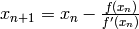
pypol.roots.newton(poly, start, epsilon=-inf)¶

Finds one root of the polynomial poly, with this iteration formula:: $x_{n + 1} = x_n - \frac{f(x_n)}{f'(x_n)}$

Parameters:	start (integer, float or complex) – the start value for evaluate `poly(x)`. epsilon (integer or float) – the precision of the calculus (default to `float('-inf')`).
Return type:	integer of float

Examples

>>> k = poly1d([2, 5, 3])
>>> k
+ 2x^2 + 5x + 3

the roots of this polynomial are -1 and -1.5. We start with 10:

>>> newton(k, 10)
-1.0000000000000002

so we try -1:

>>> newton(k, -1)
-1
>>> k(-1)
0

We have one root! We continue:

>>> newton(k, -2)
-1.5
>>> k(-1.5)
0.0

This function can find complex roots too (if start is a complex number):

>>> k = poly1d([1, -3, 6])
>>> k
+ x^2 - 3x + 6
>>> roots.quadratic(k)
((1.5+1.9364916731037085j), (1.5-1.9364916731037085j))
>>> roots.newton(k, complex(100, 1))
(1.5+1.9364916731037085j)
>>> roots.newton(k, complex(100, -1))
(1.5-1.9364916731037085j)

References

Wikipedia | MathWorld

New in version 0.3.

pypol.roots.halley(poly, start, epsilon=-inf)¶

Finds one root of the polynomial poly using the Halley’s method, with this iteration formula:: $x_{n + 1} = x_n - \frac{2f(x_n)f'(x_n)}{2[f'(x_n)]^2 - f(x_n)f''(x_n)}$

Parameters:	start (integer, float or complex) – the start value to evaluate `poly(x)` epsilon (integer or float) – the precision, default to `float('-inf')`
Return type:	integer or float

Examples

We want to find the roots of the polynomial: x^3 - 4x^2 - x - 4:

>>> p = (x + 1) * (x - 1) * (x + 4) ## its roots are: -1, 1, -4
>>> p
+ x^3 + 4x^2 - x - 4

starting from an high number:

>>> halley(p, 90)
1.0
>>> p(1.)
0.0

then we get lower:

>>> halley(p, -1)
-1.0
>>> p(-1.)
0.0

and lower:

>>> halley(p, -90)
-4.0
>>> p(-4.)
0.0

so we can say that the roots are: 1, -1, and -4.

References

Wikipedia | MathWorld

New in version 0.4.

pypol.roots.householder(poly, start, epsilon=-inf)¶

Finds one root of the polynomial poly using the Householder’s method, with this iteration formula:: $x_{n + 1} = x_n - \frac{f(x_n)}{f'(x_n)} \Big\{ 1 + \frac{f(x_n)f''(x_n)}{2[f'(x_n)]^2} \Big\}$

Parameters:	start (integer, float or complex) – the start value to evaluate `poly(x)` epsilon (integer or float) – the precision, default to `float('-inf')`
Return type:	integer or float

Examples

Let’s find the roots of the polynomial x^4 + x^3 - 5x^2 + 3x:

>>> p = (x + 3) * (x - 1) ** 2 * x
>>> p
+ x^4 + x^3 - 5x^2 + 3x
>>> householder(p, 100)
1.0000000139750058
>>> householder(p, 2)
1.0000000140746257
>>> r = householder(p, 2)
>>> p(r)
0.0
>>> householder(p, -100)
-3.0
>>> r = householder(p, -100)
>>> p(r)
0.0

if the precision is lower, the result will be worse:

>>> householder(p, 100, 0.1)
1.0623451865071678
>>> householder(p, 100, 0.00001)
1.0000036436860307
>>> householder(p, 100, 0.00000001)
1.0000000049370159
>>> householder(p, -100, 0.1)
-3.0000022501789867
>>> householder(p, -100, 0.001)
-3.0

References

Wikipedia | MathWorld

New in version 0.4.

pypol.roots.schroeder(poly, start, epsilon=-inf)¶

Finds one root of the polynomial poly using the Schröder’s method, with the iteration formula:: $x_{n + 1} = x_n - \frac{f(x_n)f'(x_n)}{[f'(x_n)]^2 - f(x_n)f''(x_n)}$

Parameters:	start (integer, float or complex) – the start value to evaluate `poly(x)` epsilon (integer or float) – the precision, default to `float('-inf')`
Return type:	integer or float

Examples

>>> k = poly1d([3, -4, -1, 4])
>>> k
+ 3x^3 - 4x^2 - x + 4
>>> schroeder(k, 100)
-0.859475828371609
>>> k(schroeder(k, 100))
0.0
>>> schroeder(k, 100j)
(1.0964045808524712-0.5909569632973221j)
>>> k(schroeder(k, 100))
-1.1102230246251565e-16j
>>> schroeder(k, -100j)
(1.0964045808524712+0.5909569632973221j)
>>> k(schroeder(k, 100))
1.1102230246251565e-16j

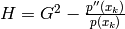
pypol.roots.laguerre(poly, start, epsilon=-inf)¶

Finds one root of the polynomial poly using the Laguerre’s method, with the iteration formula:: $x_{k + 1} = x_k - \frac{n}{max[G \pm \sqrt{(n - 1)(nH - G^2)}]}$

where:

$G = \frac{p'(x_k)}{p(x_k)}$

$H = G^2 - \frac{p''(x_k)}{p(x_k)}$

Parameters:	start (integer, float or complex) – the start value to evaluate `poly(x)` epsilon (integer or float) – the precision, default to `float('-inf')`
Return type:	complex

Examples

>>> k = poly1d([32, -123, 43, 2])
>>> k
+ 32x^3 - 123x^2 + 43x + 2
>>> laguerre(k, 100)
(3.448875873899064+0j)
>>> k(laguerre(k, 100))
(2.5579538487363607e-13+0j)
>>> laguerre(k, 1)
(0.43639990661090833+0j)
>>> k(laguerre(k, 1))
0j
>>> laguerre(k, -100)
(-0.041525780509971674+0j)
>>> k(laguerre(k, -100))
0j

pypol.roots.muller(poly, x_k, x_k2=None, x_k3=None, epsilon=-inf)¶

Finds the real roots of the polynomial poly starting from x_k.

Parameters:	x_k2 (number (integer or float)) – an optional starting value x_k3 (number (integer or float)) – another optional starting value epsilon (float) – the precision. Default to float(‘-inf’), which means it will be as accurate as possible
Return type:	number

Examples

>>> a = x.from_roots([1, -23, 2424, -2])
>>> a
+ x^4 - 2400x^3 - 58155x^2 - 50950x + 111504
>>> muller(a, 100)
-2.0
>>> muller(a, -1000)
2424.0

Muller’s method is the most suitable for a function that finds all the roots of a polynomial:

>>> def find_roots(poly):
    r = []
    for _ in xrange(poly.degree):
        next_root = muller(poly, 100)
        r.append(next_root)
        poly /= (x - next_root)
    return r

>>> find_roots(a)
[-2.0, -23.0, 2424.0, 1.0]
>>> roots.quartic(a)
[1, 2424.0, -23.0, -2.0]
>>> a = x.from_roots([1, -1, 2323, -229, 24])
>>> a
+ x^5 - 2118x^4 - 481712x^3 + 12769326x^2 + 481711x - 12767208
>>> find_roots(a)
[1.0, -1.0, -229.0, 2323.0, 24.0]

With this function you can find the roots of polynomials of higher degrees:

>>> a = x.from_roots([1, -1, 2323, -229, 24, -22])
>>> a
+ x^6 - 2096x^5 - 528308x^4 + 2171662x^3 + 281406883x^2 - 2169566x - 280878576
>>> find_roots(a)
[-22.0, 1.0, -1.0, -229.0, 2323.0, 24.0]

New in version 0.5.

pypol.roots.ridder(poly, x0, x1, epsilon=1e-09)¶

Finds the roots of the polynomial poly. Requires two starting points: x0 and x1.

Parameters:	epsilon – the precision. Default to 1e-9. The smaller epsilon is, the more accurate the calculus.
Raises :	`ValueError` is the root is not bracketed in the interval $[x0, x1]$
Return type:	number (integer or float)

Examples

>>> a = x.from_roots([1, -232, 42])
>>> ridder(a, 100, -1)
Traceback (most recent call last):
  File "<pyshell#49>", line 1, in <module>
    ridder(a, 100, -1)
  File "roots.py", line 691, in ridder
    r = []
ValueError: root is not bracketed

We have to choose the two starting values so that the root is bracketed:

>>> ridder(a, 100, 1)
1
>>> a /= (x - 1)
>>> a
+ x^2 + 190x - 9744
>>> ridder(a, 100, 1)
41.99999999999998
>>> ridder(a, 42, 1)
42
>>> a /= (x - 42)
>>> a
+ x + 232
>>> ridder(a, 100, -1000)
-232.0

New in version 0.5.

6.3. Other methods¶

pypol.roots.durand_kerner(poly, start=(0.4 + 0.9j), epsilon=1.12e-16)¶

The Durand-Kerner method. It finds all the roots of the polynomials poly simultaneously. With some polynomials it works quite well:

>>> from pypol.funcs import from_roots
>>> p = from_roots([1, -3, 14, 5, -100])
>>> p
+ x^5 + 83x^4 - 1671x^3 + 3097x^2 + 19490x - 21000
>>> durand_kerner(p)
((1+0j), (5+0j), (-100+0j), (-3+0j), (13.999999999999998+0j))
>>> map(p, durand_kerner(p))
[0j, 0j, 0j, 0j, (-7.5669959187507629e-10+0j)]
>>> p = from_roots([1, -3, 14, 5, -10, 4242])
>>> p
+ x^6 - 4249x^5 + 29553x^4 + 598609x^3 - 2064094x^2 - 7468020x + 8908200
>>> durand_kerner(p)
((1+0j), (-3+0j), (-10+0j), (5+0j), (4242-1.2727475858741762e-49j), (14+0j))
>>> map(p, durand_kerner(p))
[0j, 0j, 0j, 0j, (60112-1.7453195261352414e-31j), 0j]
>>> p = poly1d([1, 2, -3, 1, -4])
>>> durand_kerner(p)
((1.3407787867177585-9.656744866722633e-34j), (-0.084897978584602823-0.96623889223617843j), (-3.1709828295485529+8.2085042293591779e-34j), (-0.084897978584602823+0.96623889223617843j))
>>> map(p, durand_kerner(p))
[(-8.8817841970012523e-16-1.2923293554560813e-32j), (-4.4408920985006262e-16-2.2204460492503131e-16j), (3.5527136788005009e-15-3.8729295219100667e-32j), (-4.4408920985006262e-16+2.2204460492503131e-16j)]
>>> durand_kerner(p)
((1+0j), (-2424+6.2230152778611417e-61j), (14+1.2446030555722283e-60j), (381.99999999999994+4.6672614583958563e-61j), (133-7.0008921875937844e-61j), (5-2.4892061111444567e-60j), (-100+3.3735033418337674e-80j), (-3+4.9784122222889134e-60j))
>>> map(p, durand_kerner(p))
[0j, (116436291584-3.6076395061767809e-37j), 3.0129989385594897e-47j, (-110296.125+3.1986819282098692e-42j), (212+2.8399399457319209e-44j), 8.8231056584250621e-48j, 1.032541429306196e-63j, -3.3300895740082056e-47j]

But with other polynomials it could raise an OverflowError:

>>> p = poly1d([-1, 2, -3, 1, 4])
>>> p
- x^4 + 2x^3 - 3x^2 + x + 4
>>> durand_kerner(p)
Traceback (most recent call last):
  File "<pyshell#20>", line 1, in <module>
    durand_kerner(p)
  File "roots.py", line 641, in durand_kerner
    >>> map(p, durand_kerner(p))
  File "core.py", line 1429, in __call__
    return eval(self.eval_form, letters)
  File "<string>", line 1, in <module>
OverflowError: complex exponentiation

In this cases you can use other root-finding algorithms, like laguerre() or halley():

>>> laguerre(p, 10)
(5.0000000000018261+0j)
>>> laguerre(p, 5)
(5+0j)
>>> p((5+0j))
0j
>>> halley(p, 10)
5.0
>>> halley(p, 100)
14.0
>>> halley(p, 1000)
382.0
>>> halley(p, -1000)
-100.0
>>> halley(p, -100)
-100.0
>>> halley(p, -10)
-3.0

pypol.roots.brent(poly, a, b, epsilon=-inf)¶

Finds a root of the polynomial poly, with the Brent’s method.

Parameters:	a,b – The limits of the interval, where the root is searched epsilon – The precision, default to float(‘-inf’)
Return type:	integer or float

Examples

>>> p = poly1d([1, -4, 3, -4])
>>> p
+ x^3 - 4x^2 + 3x - 4
>>> brent(p, 100, -100)
3.4675038570565078
>>> r = brent(p, 100, -100)
>>> p(r)
-1.1723955140041653e-13

If we start closer:

>>> r = brent(p, 10, -10)
>>> p(r)
-1.7763568394002505e-15

the precision is greater.

References

Pseudocode from Wikipedia

Warning

Doesn’t seem to work in some cases.

pypol.roots.bisection(poly, k=0.5, epsilon=-inf)¶

Finds the root of the polynomial poly using the bisection method. When it finds the root, it checks if -root is one root too. If so, it returns a two-length tuple, else a tuple with one root.

Parameters:	k (float) – the increment of the two extreme point. The increment is calculated with the formula `a + ak`.

So, if a is 50, after the increment 50 + 50*0.5 a will be 75. epsilon sets the precision of the calculation. Smaller it is, greater is the precision.

Raises :	`ValueError` if epsilon is bigger than 5 or k is negative
Return type:	integer or float or NotImplemented when: poly has more than one letter or the root is a complex number

References

Wikipedia

Warning

In some case this function may not work!

New in version 0.2.

Changed in version 0.3.

6. The `roots` module¶

6.1. Simple algorithms and formulas¶

6.2. Newton’s method and derived¶

6.3. Other methods¶

Table Of Contents

Previous topic

Next topic

This Page

Navigation

6. The roots module¶

6.1. Simple algorithms and formulas¶

6.2. Newton’s method and derived¶

6.3. Other methods¶

Table Of Contents

Previous topic

Next topic

This Page

Quick search

Navigation

6. The `roots` module¶