Overview¶

Domain¶

A domain in pyofss contains the temporal and spectral axis (arrays) which are used by the system modules during simulation. There are helper functions which convert between frequency, angular frequency, and wavelength.

TB – total bits

SPB – samples per bit

BW – bit width

TS – total samples (TS = TB x SPB)

TW – time window (TW = TB x BW)

Using $\Delta t_{max} \equiv TW$ and $N \equiv TS$ , the temporal array corresponding to $t \in [0, \Delta t_{max})$ is generated from

$\Delta t &= \Delta t_{max} / N \\ t_n &= n \Delta t \qquad n \in [0, N)$

The first and last elements of the temporal array will have the values:

$t[0] &= 0.0 \\ t[N-1] &= \Delta t_{max} - \Delta t$

For the spectral array there will be a fixed shift such that the middle of the array corresponds to a central frequency $\nu_c$ . Then the spectral array corresponding to $\nu \in \left[ \nu_c - \frac{ \Delta \nu_{max} }{ 2 }, \nu_c + \frac{ \Delta \nu_{max} }{ 2 } \right)$ is generated from

$\Delta \nu &= \frac{ 1 }{ \Delta t_{max} } \\ \Delta \nu_{max} &= N \Delta \nu \\ \nu_n &= \nu_c - \frac{ \Delta \nu_{max} }{ 2 } + n \Delta \nu \qquad n \in [0, N)$

The first and last elements of the spectral array will have the values:

$\nu[0] &= \nu_c - \frac{ \Delta \nu_{max} }{ 2 } \\ \nu[N-1] &= \nu_c + \frac{ \Delta \nu_{max} }{ 2 } - \Delta \nu$

An angular frequency array and a wavelength array are also generated using the following two relations

$\omega &= 2 \pi \nu \\ \lambda &= c / \nu$

Field¶

The field in pyofss represents the complex valued slowly varying envelope of the electric field that will be propagated through the optical fibre system. A fixed polarisation is used for the field. It is possible to use separate field arrays for each frequency/wavelength (channel) to be simulated.

Modules¶

A module in pyofss is a class that may be called with a domain and a field as parameters. The following modules may be generated:

Gaussian¶

$A(0,t) = \sqrt{P_0} \, \exp \left[ \frac{ -(1+iC) }{ 2 } \left( \ \frac{ t-t_0 }{ \Delta t_{1/e} } \ \right)^{2m} + i \left( \phi_0 - \ 2 \pi (\nu_c + \nu_\text{offset})t \ \right) \right]$

The gaussian module will generate a (super-)Gaussian shaped pulse using the following parameters:

$P_0$ – Peak power (W)

$C$ – Chirp parameter (rad)

$t_0$ – pulse position (ps)

$\Delta t_{1/e}$ – pulse HWIeM width (ps) [note: not FWHM]

$m$ – Order paramater

$\phi_0$ – initial phase (rad)

$\nu_c$ – centre frequency (THz)

$\nu_\text{offset}$ – offset frequency (THz)

Since the centre frequency $\nu_c$ is fixed by the domain, only the offset frequency $\nu_\text{offset}$ is provided by the user.

The pulse position $t_0$ is given as a factor of the time window $\Delta t_{max}$ such that $t_0 = f \Delta t_{max}$ , and the user supplies the factor $f$ .

Sech¶

$A(0,t) = \sqrt{P_0} \, \text{sech} \left( \ \frac{ t-t_0 }{ \Delta t_{1/e} } \right) \ \, \exp \left[ \frac{ -iC }{ 2 } \left( \ \frac{ t-t_0 }{ \Delta t_{1/e} } \ \right)^2 + i \left( \phi_0 - \ 2 \pi (\nu_c + \nu_\text{offset}) t \ \right) \right]$

The sech module will generate a hyperbolic-Secant shaped pulse using the following parameters:

$P_0$ – Peak power (W)

$C$ – Chirp parameter (rad)

$t_0$ – pulse position (ps)

$\Delta t_{1/e}$ – pulse HWIeM width (ps) [note: not FWHM]

$\phi_0$ – initial phase (rad)

$\nu_c$ – centre frequency (THz)

$\nu_\text{offset}$ – offset frequency (THz)

Since the centre frequency $\nu_c$ is fixed by the domain, only the offset frequency $\nu_\text{offset}$ is provided by the user.

The pulse position $t_0$ is given as a factor of the time window $\Delta t_{max}$ such that $t_0 = f \Delta t_{max}$ , and the user supplies the factor $f$ .

Generator¶

A generator module can generate Gaussian or hyperbolic-secant (Sech) shaped pulses. The main difference to directly calling a Gaussian or Sech module is that the pulse position paramter $t_0$ is given as a factor of the bit width, and not as a factor of the time window. The user provides the factor $f$ where $t_0 = f \Delta t_{bit}$ .

Fibre¶

The fibre module propagates the input field incrementally using the generalised non-linear Schrödinger equation:

$\frac{ \partial{A} }{ \partial{z} } = \left[ \hat{L} + \ \hat{N}\left(A\right) \right] A$

where $A$ is the complex field envelope of the pulse and $z$ is the dimension along the fibre length. The linear operator $\hat{L}$ and non-linear operator $\hat{N}$ are usually written:

$\hat{L} = -\frac{\alpha}{2} - \frac{i\beta_2}{2} \ \frac{\partial^2}{\partial t^2} + \frac{\beta_3}{6} \ \frac{\partial^3}{\partial t^3} + \ldots$

$\hat{N} = i \gamma \left( |A|^2 + \frac{i}{\omega_0} \frac{1}{A} \ \frac{\partial |A|^2 A}{\partial t} - \ t_R \frac{\partial |A|^2}{\partial t} \right)$

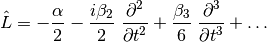
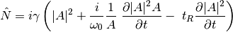
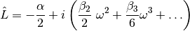
The linear operator contains terms for attenuation and (second order and higher) dispersion. The nonlinear operator contains terms for self-phase modulation (SPM), self-steepening, and Raman scattering.

It is useful to apply the linear operator to the field in the frequency domain using the property $\frac{\partial A}{\partial t} \leftrightarrow -i \omega \tilde{A}$ :

$\hat{L} = - \frac{ \alpha }{ 2 } + i \left( \frac{ \beta_2 }{ 2 } \ \omega^2 + \frac{ \beta_3 }{ 6 } \omega^3 + \ldots \right)$

Filter¶

$H(\nu) = \exp \left[ \left(\frac{- 2 \pi \ \nu_\text{filter}}{2 \Delta \nu} \right)^{2m} \right]$

The filter module will slice a specified band of the current field in the spectral domain.

Amplifier¶

$\tilde{A}_\text{out} = \sqrt{G} \tilde{A}_\text{in}$

The amplifier module applies a gain to the input field.

Overview¶

Domain¶

Field¶