4. Fibre

Note

It is assumed that pyofss has been imported using

>>> from pyofss import *

The fibre module may be regarded as the core of pyofss.

A default fibre may be generated using

>>> fibre = Fibre()

For a more interesting fibre, modify the nonlinear parameter

>>> fibre = Fibre( gamma = 1.0 )

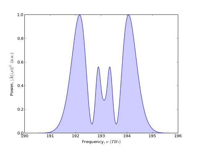
With an input pulse with sufficient power, there should be spectral broadening

from pyofss import *
sys = System()
sys.add( Gaussian(peak_power = 10.0, width = 1.0) )
sys.add( Fibre(gamma = 1.0) )
sys.run()
single_plot( sys.domain.nu, spectral_power(sys.field, True),
             labels['nu'], labels['P_nu'] )

(Source code, png, hires.png, pdf)

General dispersion may be included using the beta parameter. For third-order dispersion pass an array with third element (including a zeroth element) non-zero

>>> fibre = Fibre( beta = [0.0, 0.0, 0.0, 1.0] )

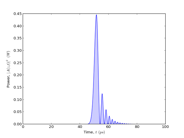
With an appropriate length of fibre the dispersion effects may be seen

from pyofss import *
sys = System()
sys.add( Gaussian(peak_power = 1.0, width = 1.0) )
sys.add( Fibre(beta = [0.0, 0.0, 0.0, 1.0], length = 10.0) )
sys.run()
single_plot( sys.domain.t, temporal_power(sys.field),
             labels['t'], labels['P_t'] )

(Source code, png, hires.png, pdf)