Joint Distributions
This is a brief introduction to working with Joint Distributions from the prob140 library. Make sure you have read the other tutorial first.
Table of Contents
Getting Started
As always, this should be the first cell if you are using a notebook.
# HIDDEN

from datascience import *
from prob140 import *
%matplotlib inline
import matplotlib.pyplot as plt
import numpy as np
plt.style.use('fivethirtyeight')
Constructing Joint Distributions
A joint distribution of multiple random variables gives the probabilities of each individual random variable taking on a specific value. For this class, we will only be working on joint distributions with two random variables.
Distribution basics
We can construct a joint distribution by starting with a Table. Calling Table().domain() with two lists will create a Table with X and Y taking on those values
In [1]: from prob140 import *

In [2]: dist = Table().domain(make_array(2, 3), np.arange(1, 6, 2))

In [3]: dist
Out[3]:
X    | Y
2    | 1
2    | 3
2    | 5
3    | 1
3    | 3
3    | 5
We can then assign values using .probability() with an explicit list of probabilities
In [4]: dist = dist.probability([0.1, 0.1, 0.2, 0.3, 0.1, 0.2])

In [5]: dist
Out[5]:
X    | Y    | Probability
2    | 1    | 0.1
2    | 3    | 0.1
2    | 5    | 0.2
3    | 1    | 0.3
3    | 3    | 0.1
3    | 5    | 0.2
To turn it into a Joint Distribution object, call the .toJoint() method
In [6]: dist.toJoint()
Out[6]:
     X=2  X=3
Y=5  0.2  0.2
Y=3  0.1  0.1
Y=1  0.1  0.3
By default, the joint distribution will display the Y values in reverse. To turn this functionality off, use the optional parameter reverse=False
In [7]: dist.toJoint(reverse=False)
Out[7]:
     X=2  X=3
Y=1  0.1  0.3
Y=3  0.1  0.1
Y=5  0.2  0.2
Naming the Variables
When defining a distribution, you can also give a name to each random variable rather than the default ‘X’ and ‘Y’. You must alternate between strings and lists when calling domain
In [8]: heads_table = Table().domain("H1",[0.2,0.9],"H2",[2,1,0]).probability(make_array(.75*.04, .75*.32,.75*.64,.25*.81,.25*.18,.25*.01))

In [9]: heads_table
Out[9]:
H1   | H2   | Probability
0.2  | 2    | 0.03
0.2  | 1    | 0.24
0.2  | 0    | 0.48
0.9  | 2    | 0.2025
0.9  | 1    | 0.045
0.9  | 0    | 0.0025

In [10]: heads = heads_table.toJoint(reverse=False)

In [11]: heads
Out[11]:
      H1=0.2  H1=0.9
H2=0    0.48  0.0025
H2=1    0.24  0.0450
H2=2    0.03  0.2025
You can also use strings for the values of the domain
In [12]: coins_table = Table().domain("Coin1",['H','T'],"Coin2", ['H','T']).probability(np.array([0.24, 0.36, 0.16, 0.24]))

In [13]: coins = coins_table.toJoint(reverse=False)

In [14]: coins
Out[14]:
         Coin1=H  Coin1=T
Coin2=H     0.24     0.16
Coin2=T     0.36     0.24
Probability Functions
We can also use a joint probability function that will take in the values of the random variables
In [15]: def joint_func(dice1, dice2):
....: return (dice1 + dice2)/252
....:
In [16]: dice = Table().domain("D1", np.arange(1,7),"D2", np.arange(1,7)).probability_function(joint_func).toJoint()
In [17]: dice
���������������������������������������������������������������������������������������������������������������������������������������������������������������������������������������������������������������������������������������������������������������������������������������������������������������������������������������������������������������������������������������������������������������������������������������������������������������������������������������������������������������������������������������������������������������������������������������������������������������������������������������������������������������Out[17]:
D1=1 D1=2 D1=3 D1=4 D1=5 D1=6
D2=6 0.027778 0.031746 0.035714 0.039683 0.043651 0.047619
D2=5 0.023810 0.027778 0.031746 0.035714 0.039683 0.043651
D2=4 0.019841 0.023810 0.027778 0.031746 0.035714 0.039683
D2=3 0.015873 0.019841 0.023810 0.027778 0.031746 0.035714
D2=2 0.011905 0.015873 0.019841 0.023810 0.027778 0.031746
D2=1 0.007937 0.011905 0.015873 0.019841 0.023810 0.027778
Marginal Distributions
To see the marginal distribution of a variable, call the method .marginal(label) where label is the string of the label
In [18]: heads.marginal("H1")
Out[18]:
H1=0.2 H1=0.9
H2=0 0.48 0.0025
H2=1 0.24 0.0450
H2=2 0.03 0.2025
Sum: Marginal of H1 0.75 0.2500
In [19]: heads.marginal("H2")
����������������������������������������������������������������������������������������������������������������������������������������������������������������������������������������������Out[19]:
H1=0.2 H1=0.9 Sum: Marginal of H2
H2=0 0.48 0.0025 0.4825
H2=1 0.24 0.0450 0.2850
H2=2 0.03 0.2025 0.2325
In [20]: coins.marginal("Coin1")
��������������������������������������������������������������������������������������������������������������������������������������������������������������������������������������������������������������������������������������������������������������������������������������������������������������������������������������������������������������������������������Out[20]:
Coin1=H Coin1=T
Coin2=H 0.24 0.16
Coin2=T 0.36 0.24
Sum: Marginal of Coin1 0.60 0.40
You can also call .both_marginals() to see both marginal distributions at once
In [21]: heads.both_marginals()
Out[21]:
H1=0.2 H1=0.9 Sum: Marginal of H2
H2=0 0.48 0.0025 0.4825
H2=1 0.24 0.0450 0.2850
H2=2 0.03 0.2025 0.2325
Sum: Marginal of H1 0.75 0.2500 1.0000
In [22]: coins.both_marginals()
�������������������������������������������������������������������������������������������������������������������������������������������������������������������������������������������������������������������������������������������������������������������������������������������������������Out[22]:
Coin1=H Coin1=T Sum: Marginal of Coin2
Coin2=H 0.24 0.16 0.4
Coin2=T 0.36 0.24 0.6
Sum: Marginal of Coin1 0.60 0.40 1.0
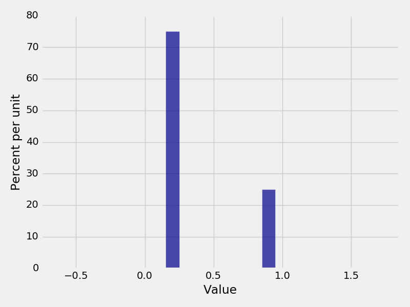
To get the marginal distribution of a variable as a single variable distribution for plotting, call .marginal_dist(label)
In [23]: heads.marginal_dist("H1")
Out[23]:
Value | Probability
0.2   | 0.75
0.9   | 0.25
In [24]: Plot(heads.marginal_dist("H1"), width=0.1)
In [25]: heads.marginal_dist("H2")
Out[25]:
Value | Probability
0 | 0.4825
1 | 0.285
2 | 0.2325
In [26]: coins.marginal_dist("Coin1")
��������������������������������������������������������������������������Out[26]:
Value | Probability
H | 0.6
T | 0.4
Conditional Distributions
You can see the conditional distribution using .conditional_dist(label, given). For example, to see the distribution of H1|H2, call .conditional_dist(“H1”, “H2”)
In [27]: heads.conditional_dist("H1", "H2")
Out[27]:
H1=0.2 H1=0.9 Sum
Dist. of H1 | H2=0 0.994819 0.005181 1.0
Dist. of H1 | H2=1 0.842105 0.157895 1.0
Dist. of H1 | H2=2 0.129032 0.870968 1.0
Marginal of H1 0.750000 0.250000 1.0
In [28]: heads.conditional_dist("H2", "H1")
��������������������������������������������������������������������������������������������������������������������������������������������������������������������������������������������������������������������������������������Out[28]:
Dist. of H2 | H1=0.2 Dist. of H2 | H1=0.9 Marginal of H2
H2=0 0.64 0.01 0.4825
H2=1 0.32 0.18 0.2850
H2=2 0.04 0.81 0.2325
Sum 1.00 1.00 1.0000