Basic fcm tutorial
Loading fcs data
fcm provides the loadFCS() function to load fcs files:
>>> from fcm import loadFCS
>>> data = loadFCS('../sample_data/3FITC_4PE_004.fcs')
>>> data
3FITC_4PE_004
>>> data.channels
['FSC-H', 'SSC-H', 'FL1-H', 'FL2-H']
>>> data.shape
(94569, 4)
Since the FCMdata object returned by loadFCS() delegates to underlying numpy array, you can pass the FCMdata object to most numpy functions
>>> import numpy as np
>>> np.mean(data)
410.38791252947584
>>> np.mean(data,0)
array([ 538.76464803, 421.57733507, 340.03599488, 341.17367213])
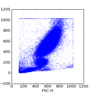
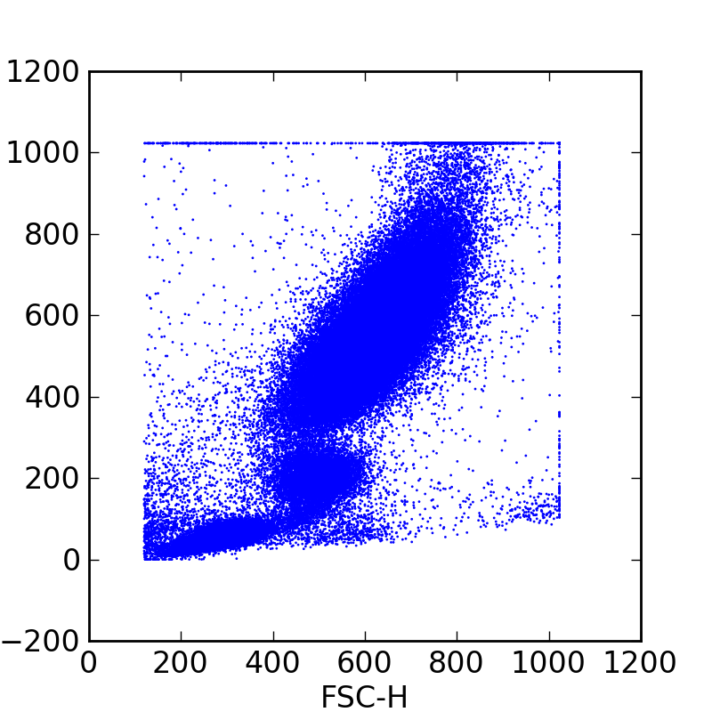
>>> import pylab
>>> pylab.scatter(data[:,0],data[:,1], s=1, edgecolors='none')
>>> pylab.xlabel(data.channels[0])
>>> pylab.ylabel(data.channels[1])
>>> pylab.show()
(Source code, png, hires.png, pdf)

FCMdata objects also provide some basic Q/A via the FCMdata.summary() method which shows the means, and standard deviations of each channel, along with the FCMdata.boundary_events() method to inspect the number of events along the boundaries.
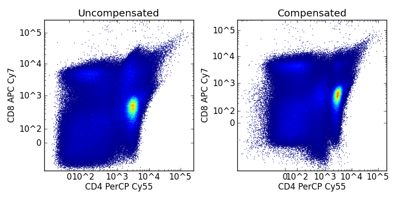
Compensation and Transformation
Along with reading FCS files, fcm provides methods to apply compensation to try and counter fluorescent spill over. By default loadFCS() compensates fcs data using the compensation matrix provided in fcs file header. loadFCS() also allows you to provide your own compensation matrix by passing in the comp and sidx arguments, or can not compensate by passing False as the auto_comp argument to loadFCS(). For convenience fcm provides the load_compensate_matrix() which will return the laser names (sidx) and compensation matrix exported in the format used by Flowjo.
fcm also supports the logicle and log data transforms. By default when loading an fcs file loadFCS() will apply the logicle transform to all fluorescent channels with a range of 262144 (PNR in the fcs header). The log transform can be used instead by passing the transform argument of log or automatic transformation can be prevented by setting the transform argument to None.
Further FCMdata provides FCMdata.compensate(), FCMdata.logicle(), and FCMdata.log() methods. The code below shows how to control and manually apply logicle transforms and compensation to a FCMdata object. It also shows the basics of working with the FCMdata data tree which will be covered in the next section
import fcm
import fcm.graphics as graph
import matplotlib.pyplot as pylab

sidx, comp = fcm.load_compensate_matrix('CompMatrixDenny06Nov09')

data = fcm.loadFCS('E6901F0T-07_CMV pp65.fcs', auto_comp=False, transform=None)

data.logicle() # logicle the data so it looks more like you are used to seeing
data.tree.rename_node('t1','uncompensated')

data.visit('root')
data.compensate(sidx,comp)
data.logicle()
data.tree.rename_node('t1','compensated')


fig = pylab.figure(figsize=(8,4))
ax = pylab.subplot(1,2,1)

data.visit('uncompensated')
z = graph.bilinear_interpolate(data[:,'CD8 APC Cy7'],data[:,'CD4 PerCP Cy55'])
ax.scatter(data[:,'CD4 PerCP Cy55'],data[:,'CD8 APC Cy7'], s=1, edgecolor='none', c=z)
ax.set_xlabel('CD4 PerCP Cy55')
ax.set_ylabel('CD8 APC Cy7')
graph.set_logicle(ax,'x')
graph.set_logicle(ax,'y')
ax.set_xlim(-7000, data[:,'CD4 PerCP Cy55'].max())
ax.set_ylim(-9000, data[:,'CD8 APC Cy7'].max())
ax.set_title('Uncompensated')

ax = pylab.subplot(1,2,2)

data.visit('compensated')

z = graph.bilinear_interpolate(data[:,'CD8 APC Cy7'],data[:,'CD4 PerCP Cy55'])
ax.scatter(data[:,'CD4 PerCP Cy55'],data[:,'CD8 APC Cy7'], s=1, edgecolor='none', c=z)
ax.set_xlabel('CD4 PerCP Cy55')
ax.set_ylabel('CD8 APC Cy7')
graph.set_logicle(ax,'x')
graph.set_logicle(ax,'y')
ax.set_xlim(-30000, data[:,'CD4 PerCP Cy55'].max())
ax.set_ylim(-30000, data[:,'CD8 APC Cy7'].max())
ax.set_title('Compensated')

print data.tree.pprint()
pylab.tight_layout()
fig.savefig('comp.png')
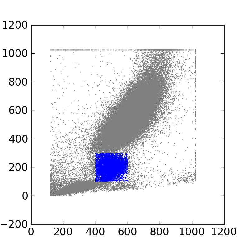
Gating and working withe the view tree
Typical flow analysis focuses on finding cell subsets of interest via gating. fcm has objects representing several types of gates, PolyGate, QuadGate, IntervalGate, and ThresholdGate, in addition to gate like filter objects, Subsample, and DropChannel
The view Tree manages the subsets of the original fcs file data as we define new subsets by gating or filtering. To look at the structure of the tree, you can get the current node by the FCMdata.current_node() and to view the layout of the tree use the FCMdata.tree.pprint() method, and to move to different nodes in the tree use either the FCMdata.visit() or FCMdata.tree.visit() methods.
import fcm
import matplotlib.pyplot as plt

#load FCS data
data = fcm.loadFCS('3FITC_4PE_004.fcs')

#define a gate
gate1 = fcm.PolyGate([(400,100),(400,300),(600,300),(600,100)], (0,1))

#apply the gate
gate1.gate(data)

# outputs:
# root
#    g1
print data.tree.pprint()

# g1 isn't and informative name, so lets rename it events
current_node = data.current_node
data.tree.rename_node(current_node.name, 'events')
# outputs:
# root
#    events
print data.tree.pprint()

#return to the transformed node and plot
data.tree.visit('root')
plt.figure(figsize=(4,4))
plt.scatter(data[:,0],data[:,1], s=1, edgecolors='none', c='grey')

#and visit the subset of interest to plot
data.tree.visit(current_node)
plt.scatter(data[:,0],data[:,1], s=1, edgecolors='none', c='blue')
plt.show()
(Source code, png, hires.png, pdf)

Chaining Commands
Since most methods on FCMdata return itself you can chain commands together one after another. for example
>>> data.gate(g1).gate(g2).gate(g3)
Working with collections
Since often the same analysis is applied to several fcs files, fcm has a FCMcollection object with methods that apply to each file in the collection. Below is an example of loading several files, and applying a common gate to each of them.
>>> data1 = loadFCS('file1.fcs')
>>> data2 = loadFCS('file2.fcs')
>>> data3 = loadFCS('file3.fcs')
>>> collection = FCMcollection('test',[data1, data2, data3])
>>> print collection.keys()
['file1','file2','file3']
>>> collection.gate(g1)
>>> print collection['file2'].tree.pprint()
root
  t1
    c1
      g1
>>> print collection['file1'].tree.pprint()
root
  t1
    c1
      g1
you can use the loadMultipleFCS() function to load several fcs files to help with building collections.