mfng - Multifractal network generator

The theoretical background can be found in the article Palla-Vicsek-Lovász: Multifractal network generator. This can be download for free. We use the K instead of k for the number of iteration, and k for degree, and we use 0-based indexing (the top row is the 0th row).

In this tutorial we suppose we use Linux or UNIX operating system to run the mfng. We think, we can use mfng on other operating systems, where Python, igraph and numpy can be installed, however we have no too much experiences.

The references of mfng and mfng.analyzer modules can be found in other pages. Those pages describes the details of the modules. The references have been created mainly from the documentation strings of the program, so they are quite up-to-date.

Usage

If we have not installed the cxnet globally we must be in the cxnet/mfng directory:

cd cxnet/mfng

We need to run a script like mfngrun.py in this directory, but we should copy it to another name. If cxnet is not installed globally, the copy must be in the same directory, else anywhere. We are allowed to run mfngrun.py directly, but if we change it, the update with bzr pull will be more complicated.

We advise to make a copy if we want to modify it. For example with the name mrun.py:

cp mfngrun.py mrun.py

We can change the mrun.py file as we want. We find help for this in the next section. Then we can run:

python mrun.py

The results will be saved in several formats in the project directory. About these files see the section Result files.

The details (the probabilities, division points and the energy in each step, and whether the step was accepted or rejected) are printed onto the screen.

This output can be redirected into a given file on UNIX and Linux systems with the command:

python mrun.py >> project_base/details.txt

So, with double greater-than sign (>>), the results will be appended to the original file. With one greater-than sign the original data will be overwritten with the new data.

The parameters in the mfngrun.py (mrun.py) file

We can use all of the features of the Python language in the mrun.py file. We write here some basic things about the Python language and the simulation.

We need to know, that in the Python the statements are grouped by indentation. While below the for-row the statements are indented the same amount, these statements belongs to the for-cycle. When a statements are indented as the for-row, this statement will be executed after the for-cycle.

An excellent tutorial of the Python programming language can be reached from the official Python site: http://docs.python.org . A good book is the Dive Into Python.

The most important parameters of the generator object (see mfng.Generator) are.

Name	description
T0	initial temperature
Tlimit	the temperature decreases until Tlimit
steps	the number of steps we want
m	the number of division point in the divs
K	number of iteration
n	the number of nodes in the generated networks
divexponent	the exponent at the changing the division points
project	the name of the project

The results will be in the project directory. Its name is the project name appended to the “project_” string. The default project name is base, so the project directory is project_base.

One or more variables can be changed by for-cycle(s), and with these different parameters run the simulation.

An arbitrary property can be append to the generator object with the generator.append_property method. If we want the average degree of the network be 20, we must append the AverageDegree property:

generator.append_property(AverageDegree(20))

We can optimize more properties in the same simulation, however not all of the variations make sense (e.g. average degree and degree distribution in the same time).

Result files

There are several result files in the project directory. The analyzer module uses the runs.shelf file. This is a binary format, that uses shelf, the standard serialization module of Python. This includes most saved information, than the other result files.

If you want to look the results as text, you can view the runs.py or the runs.json files with an editor.

The result files includes

• the more important parameters of the runs
• the given divs and probs values, and the
• how long took the run.

The runs.shelf file includes also the energy, the divs and the probs in each step.

The result files includes also a string that shows, which step was the new measure accepted or rejected in. (A= accepted with less energy, a= accepted with higher energy, . (dot)= rejected). For example here is the beginning of the accept_reject string:

accept_reject = "AA aA Aa Aa .a aA Aa A. A. A. .. ..

In the first and second step the measure was accepted, because its energy was lower than the actual energy. In the third step the measure was accepted, however its energy was more then the actual energy. In the ninth step the measure was rejected.

Analysis of the results

To the easiest way to analyze the runs, we need to go to the project directory. E.g.

cd project_base

There is a module with the name analyzer in the cxnet package. With it we can calculate and plot some of the more important properties of he given measure. We give a sample, how to use this module with ipython Python shell. In this section we suppose, we have started the ipython with the -pylab option like this:

ipython -pylab

(The standard Python shell is not able to plot several function into one plot, so not all the examples will run.) In the rows started with In [x] and Out [x] are the written statements and its returning values respectively.

In [1]: import analyzer
I have found an rc file: /home/ha/.cxnetrc.py.
The graph_module was set in the rc file to "igraph".
I will use igraph. (It have been imported.)

(The import procedure give us information, whether the igraph or the networkx will be used. For the analysis of the result of mfng we need to use igraph.)

In [2]: r=analyzer.Runs()

If we have not installed the cxnet globally we must be in the cxnet/mfng directory, the project directory must be in this directory, and we need to give the name of the project directory (project_base in the example):

In [2]: r=analyzer.Runs('project_base')
or
In [2]: r=analyzer.Runs(project='project_base')

In [3]: r.set_labels("3500_001")
Out[3]: ['3500_001']

If we runs several simulation in the same project with 3500 nodes, the label of the first run will be 3500_001, the label of the second run will be 3500_002 and so on. We need to set this label to analyze this run. We can set a list of labels. In this case the analysis go through all of the runs if it makes sense, otherwise the analysis deals only with the first label. (In Pythonban we need not care whether we use simple quote or double (' or ") to give a string; both of them has the same meaning. List can be given in square brackets, and the elements of the list are separated by a comma. E.g. ['3500_001', '3500_002'])

If we do not give any parameters to the set_labels method, i.e. we call it as r.set_labels() then we will get the list of all labels. Further reading in the mfng documantation: mfng.analyzer.Runs.set_labels.

Determination of some base properties with network generation

In [4]: r.properties(n=50)
====================
label = 3500_001
====================

number of generated networks = 50
divs = [0.90256203480899999, 1.0],
probs=[[ 0.15533352  0.31063345]
 [ 0.31063345  0.22339959]]
   avg max deg = 105.14+-9.68485036181, avg average deg=21.5726628571+-0.301747377812

In this case we have generated n=50 networks, and we got some properties of these networks.

The easiest way to determine degree distribution

If we have chosen the runs we want to investigate with the r.set_labels function, we can plot the degree distributions in loglog scale (log scale in both axes) with the statement:

In [14]: r.loglog()

We can change the title and other parameters as we will see in the section Determination of the degree distribution, the more flexible way.

Changing of the energy and the division points

We can plot the energy as the function of the step number with the method mfng.analyzer.Runs.plot_energy_list:

In [3]: r.set_labels(["2000_001", "2000_002"])
["2000_001", "2000_002"]
In [4]: r.plot_energy_list()

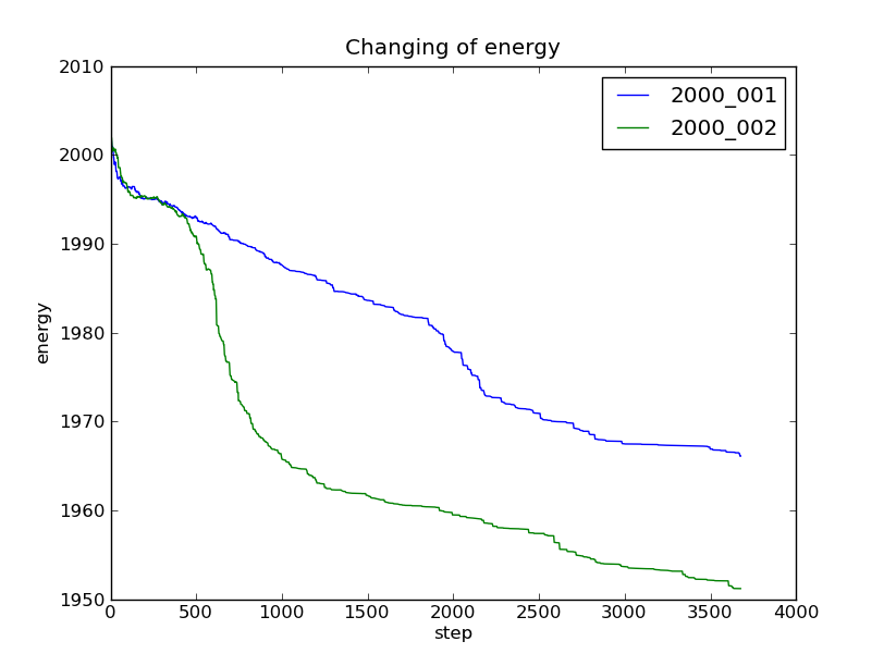
This method will plot the changing of the energy for all of the labels we have set.

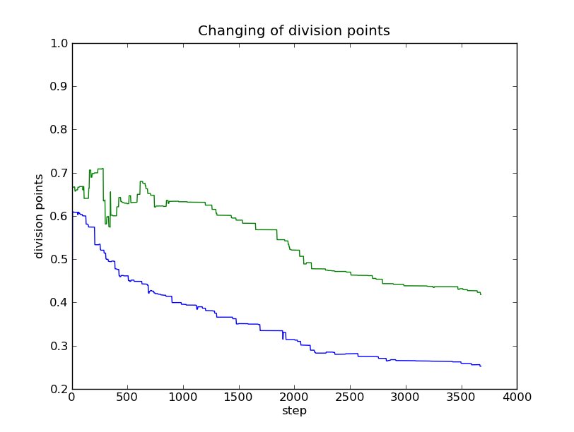
The changing of the division points can be plotted with the mfng.analyzer.Runs.plot_divs_list method. This function will plot only the changing for the first label:

In [5]: r.plot_divs_list()

Determination of the degree distribution, the more flexible way

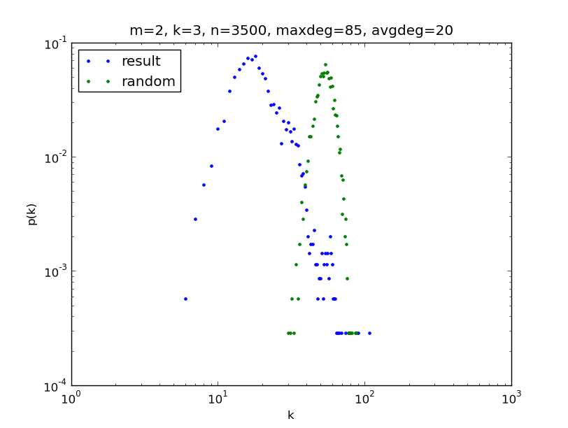
In [5]: dd=r.degdist()

This method returns with an object from the cxnet.DegreeDistribution class. Its more verbose description can be found at the documentation of the cxnet module. It should be read to understand the examples below.

In [6]: dd.set_binning("all")

In [7]: dd.loglog()
Out[7]: [<matplotlib.lines.Line2D object at 0xf8ac3ac>]

We can create a degree distribution from the original measure also, to see, what has been changed. If we started the ipython with the -pylab option, we can plot also this distribution into the same plot:

In [8]: ddi=r.degdist(initial=True) # The distribution of random network (original prob. measure)

In [9]: ddi.set_binning("all")

In [10]: ddi.loglog()
Out[10]: [<matplotlib.lines.Line2D object at 0xfe4afac>]

The matplotlib package, and its part, the pylab module give us the possibility to modify the plot. We can read the possibilities in the web page of matplotlib We can set for example the title of the plot, give comment to each plotted function, and at the and we can save the plot into a file. The vector graphical file formats has some advantages over the raster graphical ones: the pdf is good for pdflatex, and the eps for latex. If we want pixel graphics, we can choose the png format, it can be embedded into a web page. Important plots are worthwhile to save into all of the three formats:

In [11]: title("""m=2, K=3, n=3500, maxdeg=85, avgdeg=20""")
Out[11]: <matplotlib.text.Text object at 0xf8a63ac>

In [12]: legend(("result", "random"),loc="upper left")
Out[12]: <matplotlib.legend.Legend object at 0xfcb5c0c>

In [13]: savefig("3500_001degdist.pdf") # instead of pdf can be png or eps as well

The last row gives a figure like this.