cxnet Tutorial
This tutorial describes only the cxnet modul. There are also two disctinct modules (mfng and network_evolution) described in the next sections.
You can import the cxnet module as:
import cxnet
It imports igraph module or if it can not do the NetworkX module.
Without one of these modules one can have a very limited functions.
cxnet
If you use cxnet with igraph you will have a class Network. Network is a class based on igraph.Graph, so you can use all of the methods the base class has. The network (graph) generation is the same as described in the python-igraph tutorial.
Here is an example:
>>> import cxnet
I have found an rc file: /home/ha/.cxnetrc.py.
The graph_module was set in the rc file to "igraph".
I will use igraph. (It have been imported.)
>>> net = cxnet.Network()
>>> net.add_vertices(8)
>>> net.add_edges([(1,2), (2,4), (3,5)])
>>> net = cxnet.Network.Full(9)
>>> net.delete_edges([(3,4), (6,7), (0,1)])
>>> cxnet.summary(net)
IGRAPH U--- 9 33 --
>>> cxnet.plot(net, layout="circular")
<igraph.drawing.Plot object at 0x911556c>
The IGRAPH U— 9 33 – above shows that we created an undirected (U) network with 9 vertices and 33 edges.
But there are some special methods of Network. These are usually starting with cx so with the ipython shell we can find it easier. These methods are usually useful with graphs, which has vertex attribute name including the package dependency network.
Creating deb package dependency network
Note
The most of the things written in this section can be used with networkx as well.
deb packages are originally developed for the Debian distribution of GNU/Linux, but there are more distributions using it, eg. the Ubuntu variants.
On Linux distributions using deb packages you can create the dependency network of the deb packages and get its main properties this way:
>>> dn = cxnet.debnetwork()
Getting package names and dependencies.
Removing edges, which target is not in self.vertices.
Transforming to numbered graph.
Transforming to igraph.
>>> cxnet.summary(dn)
28212 nodes, 130173 edges, directed

Number of components: 27668
Diameter: 15
Density: 0.0002
Reciprocity: 0.0037
Average path length: 3.6433
You can find packages wich name includins a string with the cxfind() method:
>>> dn.cxfind("firefox")
['firefox', 'firefox-2', 'firefox-2-dbg', 'firefox-2-dev',
'firefox-2-dom-inspector', 'firefox-2-gnome-support', 'firefox-2-libthai',
'firefox-3.0', 'firefox-3.0-dev', 'firefox-3.0-gnome-support',
'firefox-3.5', 'firefox-3.5-branding', 'firefox-3.5-dbg',
'firefox-3.5-dev', 'firefox-3.5-gnome-support', 'firefox-branding',
'firefox-dbg', 'firefox-dev', 'firefox-gnome-support',
'firefox-gnome-support-dbg', 'firefox-launchpad-plugin', 'firefox-notify',
'firefox-ubuntu-it-menu', 'firefox-webdeveloper',
'kubuntu-firefox-installer']
You can find the neighbors with the cxneighbors() method. It returns a pair of lists. The first list includes the packages depending on the packages (the edges pointing to the package), the second list includes the packages the given package depends on:
>>> inn, outn = dn.cxneighbors("firefox")
>>> inn
['firefox-globalmenu', 'pytrainer', 'icedtea-plugin', 'firefox-gnome-support', 'gecko-mediaplayer', 'sugar-firefox-activity', 'mozilla-virt-viewer', 'tiemu', 'mozilla-gtk-vnc', 'wysihtml-el', 'browser-plugin-packagekit', 'chemical-structures', 'webhttrack', 'mozplugger', 'gcu-plugin', 'xul-ext-mozvoikko', 'mediatomb', 'firefox-dbg', 'deejayd-webui-extension', 'firefox-dev', 'firefox-branding', 'firefox-launchpad-plugin', 'abrowser-branding', 'abrowser']
>>> outn
['libxt6', 'libc6', 'libgcc1', 'libglib2.0-0', 'libcairo2', 'libfontconfig1', 'zlib1g', 'libstdc++6', 'libgdk-pixbuf2.0-0', 'libx11-6', 'debianutils', 'libdbus-1-3', 'libatk1.0-0', 'libfreetype6', 'libgtk2.0-0', 'libpango1.0-0', 'psmisc', 'libxext6', 'libasound2', 'libdbus-glib-1-2', 'lsb-release', 'fontconfig', 'libstartup-notification0', 'libxrender1']
(You can not use in as variable name, it is a reserved word in Python. That is why the example uses inn instead.)
We can plot the neighborhood of the given package with the cxneighborhood() method. If plot is True then we get a plot in a window, if it is a name of a file, it will be save it into that file, if it is just “pdf” “png” or “svg” it creates a file of the given format with a name like neighbors_of_firefox.pdf.
>>> dn.cxneighborhood("firefox")
<igraph.VertexSeq object at 0x94f6f7c>
>>> dn.cxneighborhood("firefox", plot="pdf")
<igraph.VertexSeq object at 0xc046374>
>>> dn.cxneighborhood("firefox", plot="firefox_neighbors.png")
<igraph.VertexSeq object at 0xc046374>
>>> vertex_seq = dn.cxneighborhood("firefox", plot=False)
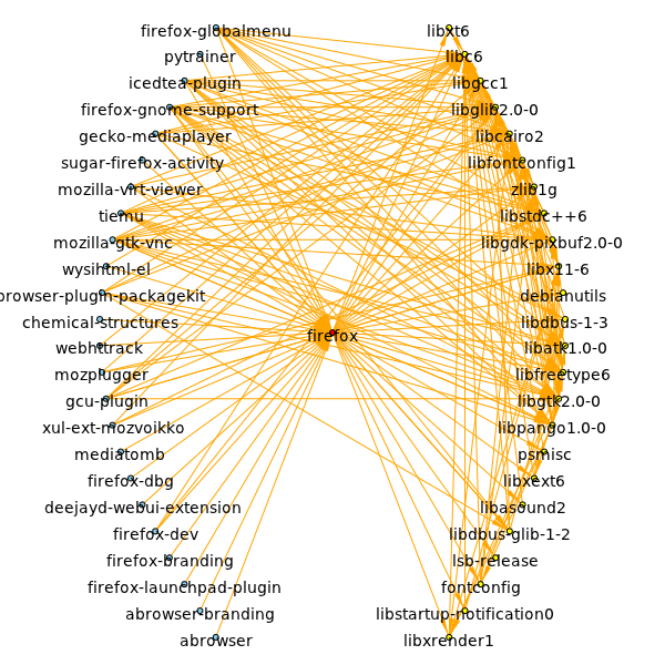
The plot we get with dn.cxneighborhood("firefox", plot="png"). The firefox package depends on the packages at right, and the packages at left depend on firefox.
Note
In the case you use networkx, you need the networkx version >= 1.2.
You can store the dependency network with the function cxwrite():
>>> dn.cxwrite()
See files 'ubuntu-11.04-packages-2011-08-31.gml', 'ubuntu-11.04-packages-2011-08-31.txt'
and 'netdata_zip/ubuntu-11.04-packages-2011-08-31.zip'.
'ubuntu-11.04-packages-2011-08-31'
We got two files with extensions .gml and .txt. The gml file can be read with cxnet, as described in the section Getting network data. The txt file contains information about the distribution and the used repositories.
You can get the vertices with the largest degrees (indegrees, outdegrees) with the cxlargest_degrees():
>>> ld = dn.cxlargest_degrees()
>>> ld
[(14161, 'libc6'), (4036, 'libstdc++6'), (3902, 'libgcc1'), (3030, 'perl'), (2784, 'libglib2.0-0'), (2639, 'python'), (1909, 'libx11-6'), (1779, 'libgtk2.0-0'), (1660, 'zlib1g'), (1384, 'python-support'), (1351, 'dpkg'), (1304, 'libpango1.0-0'), (1263, 'libcairo2'), (1208, 'libfreetype6'), (1110, 'libqtcore4'), (1079, 'libatk1.0-0'), (1075, 'libfontconfig1'), (949, 'libxml2'), (946, 'libqtgui4'), (945, 'libgdk-pixbuf2.0-0'), (892, 'debconf'), (772, 'libxext6'), (663, 'libpng12-0'), (653, 'python-central'), (591, 'libkdecore5'), (583, 'libssl0.9.8'), (578, 'libncurses5'), (504, 'adduser')]
>>> ldin = dn.cxlargest_degrees("in")
>>> ldin
[(14158, 'libc6'), (4032, 'libstdc++6'), (3899, 'libgcc1'), (3023, 'perl'), (2779, 'libglib2.0-0'), (2637, 'python'), (1905, 'libx11-6'), (1751, 'libgtk2.0-0'), (1658, 'zlib1g'), (1382, 'python-support'), (1345, 'dpkg'), (1293, 'libpango1.0-0'), (1252, 'libcairo2'), (1205, 'libfreetype6'), (1105, 'libqtcore4'), (1075, 'libatk1.0-0'), (1069, 'libfontconfig1'), (947, 'libxml2'), (938, 'libgdk-pixbuf2.0-0'), (926, 'libqtgui4'), (890, 'debconf'), (769, 'libxext6'), (660, 'libpng12-0'), (652, 'python-central'), (582, 'libkdecore5'), (580, 'libssl0.9.8'), (577, 'libncurses5'), (501, 'adduser'), (485, 'libice6'), (478, 'libsm6'), (471, 'libkdeui5'), (448, 'libgl1-mesa-glx'), (444, 'libjpeg62'), (440, 'libdbus-1-3'), (414, 'locales'), (413, 'libgconf2-4'), (411, 'libgmp3c2'), (405, 'libsdl1.2debian'), (397, 'python-gtk2'), (396, 'libqt4-xml'), (378, 'libdbus-glib-1-2'), (350, 'libqt4-dbus'), (348, 'libqt4-network'), (331, 'libkio5'), (330, 'libxt6'), (323, 'libc6-dev'), (310, 'gconf2'), (305, 'kdebase-runtime'), (303, 'lsb-base')]
DegreeDistribution class
You can create the degree distribution of a network with the cxnet.DegreeDistribution class:
>>> dd=cxnet.DegreeDistribution(dn)
With this class you can use an igraph.Graph object, a networkx.Graph object or a degree list as first parameter.
If you need indegree distribution or outdegree distribution instead, you need the direction argument:
>>> ddin =cxnet.DegreeDistribution(dn, direction="in")
>>> ddout=cxnet.DegreeDistribution(dn, direction="out")
If you expect the network is a scale-free one, you can get its exponent and its standard deviation like this:
>>> gamma, sigma = dd.exponent()
>>> gamma, sigma
(2.3182668687237862, 0.013005694686864753)
For details see the documentation of the exponent().
You can plot this distribution if pylab (matplotlib) is installed:
>>> dd.set_binning("log")
>>> dd.loglog(); dd.plot_powerlaw()
[<matplotlib.lines.Line2D object at 0xa66404c>]
[<matplotlib.lines.Line2D object at 0xa46516c>]
loglog() plots the distribution with log scales on each axes. You can use plot() (linear on each axes) or semilogy() (logaritmic on y axis) as well. plot_powerlaw() plots a powerlaw distribution with the exponent calculated by the exponent() method.
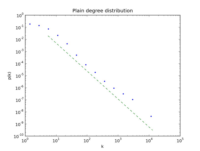
The plot we get
Getting network data
If you have Web connection, you can download data of complex networkx:
>>> cxnet.get_netdata()
You need to choose an archive name.
Use one of them:
get_netdata("newman")
get_netdata("deb")

>>> cxnet.get_netdata("newman")
karate.zip
        karate.gml, karate.txt
lesmis.zip
        lesmis.gml, lesmis.txt
(...)
This will
- create two directories into the actual directory: netdata_zip and netdata,
- download the zip files of netdata into the netdata_zip directory,
- unzip the zip files creating a gml file and a txt file from each archive.
The gml files can be read with cxnet or IGraph:
>>> net = cxnet.Network.Read("netdata/karate.gml")
or
>>> import igraph
>>> net = igraph.Graph.Read("netdata/karate.gml")