Getting started
Contents
Hi-C data format
Hi-C data are usually represented as symmetric matrices in a tab separated file, as in the example below:
chrT_001      chrT_002        chrT_003        chrT_004        chrT_005        chrT_006
chrT_001      629     164     88      105     10      35
chrT_002      86      612     175     110     40      29
chrT_003      159     216     437     105     43      73
chrT_004      100     111     146     278     70      42
chrT_005      16      36      26      79      243     39
chrT_006      19      50      53      42      37      224
TADBit allows to load most of this kind of matrices. A Hi-C matrix is loaded as this (note: this example loads human chromosome 19 from [Lieberman-Aiden2009] results.):
from pytadbit import Chromosome

# initiate a chromosome object that will store all Hi-C data and analysis
my_chrom = Chromosome(name='My first chromosome')

# load Hi-C data
my_chrom.add_experiment('First Hi-C experiment', xp_handler="sample_data/HIC_k562_chr19_chr19_100000_obs.txt", resolution=100000)
Warning
TADBit assumes that Hi-C data matrices starts at chromosome position 1. If your matrix do not represents the full chromosome length, fill the missing columns and rows with zeros.
Unconventional data format
If TADBit is unable to parse the input file, the user can create its own parser and pass it to the Chromosome instance. For example, one might be interested in using [Dixon2012] data that appear like this:
chr21 0       20000   0       0       0       0       0       0       0       0
chr21 20000   40000   0       0       0       0       0       0       0       0
chr21 40000   60000   0       0       0       0       0       0       0       0
chr21 60000   80000   0       0       0       0       0       0       0       0
chr21 80000   100000  0       0       0       0       0       0       0       0
chr21 100000  120000  0       0       0       0       0       0       0       0
chr21 120000  140000  0       0       0       0       0       0       0       0
chr21 140000  160000  0       0       0       0       0       0       0       0
In this case the user could implement a simple parser like this one:
def read_dixon_matrix(f_handle):
    """
    reads from file handler (already openned)
    """
    nums = []
    start = 3
    for line in f_handle:
        values = line.split()[start:]
        nums.append([int(v) for v in values])
    f_handle.close()
    return tuple([nums[j][i] for i in xrange(len(nums)) for j in xrange(len(nums))]), len(nums)
And call it as follow:
my_chrom.add_experiment("/some_path/hi-c_data.tsv", name='First Hi-C experiment',
                         parser=read_dixon_matrix)
Experiments, when loaded, are stored in a special kind of list attached to chromosome objects:
my_chrom.experiments
which will return:
[Experiment First Hi-C experiment (resolution: 20Kb, TADs: None, Hi-C rows: 100)]
A specific Experiment can be accessed either by its name or by its position in pytadbit.chromosome.ExperimentList :
my_chrom.experiments[0] == my_chrom.experiments["First Hi-C experiment"]
Each Experiment is an independent object with a list of associated functions (see pytadbit.experiment.Experiment).
Find Topologically Associating Domains
Once an experiment has been loaded, the location of Topologically Associating Domains (TADs) can be estimated as:
my_chrom.find_tad('First Hi-C experiment')
pytadbit.chromosome.Chromosome.find_tad() is called from our Chromosome object but is applied to a specific experiment. Therefore, TADs found by TADBbit will be associated to this specific experiment. They can be accessed as following:
exp = my_chrom.experiments["First Hi-C experiment"]
exp.tads
The “tads” variable returned in this example is a dictionary of TADs, each of each is in turn a new dictionary containing information about the start and end positions of a TAD:
{0: {'start': 0,
     'end'  : 24,
     'brk'  : 24,
     'score': 8},
 1: {'start': 25,
     'end'  : 67,
     'brk'  : 67,
     'score': 4},
 :...
 :...
 :...
 }
“start” and “end” values correspond respectively to the start and end positions of the given TAD in the chromosome (note that this numbers have to be multiplied by the resolution of the experiment, “exp.resolution”). The “brk” key corresponds to the value of “end”, all “brk” together corresponds to all TAD’s boundaries.
Forbidden regions and centromeres
Once TADs are detected by the core pytadbit.tadbit.tadbit() function, TADBit checks that they are not larger than a given value (3 Mb by default). If a TAD is larger than this value, it will be marked with a negative score, and will be automatically excluded from the main TADBit functions.
Another inspection performed by TADBit is the presence of centromeric regions. TADBit assumes that the larger gap found in a Hi-C matrix corresponds to the centromere. This search is updated and refined each time a new experiment is linked to a given Chromosome. Typically, TADs calculated by the core pytadbit.tadbit.tadbit() function include centromeric regions; if a centromere is found, TADBit will split the TAD containing it into two TADs, one ending before the centromere and one starting after. As centromeric regions are not necessarily TAD boundaries, the TADs surrounding them are marked with a negative score (as for forbidden regions).
Data visualization
Once loaded, the Hi-C data can be visualized using the pytadbit.chromosome.Chromosome.visualize() function. The only parameter needed is which experiment to show. Therefore, the human chromosome 19 from [Lieberman-Aiden2009] can be visualized with:
my_chrom.visualize("First Hi-C experiment", show=True)
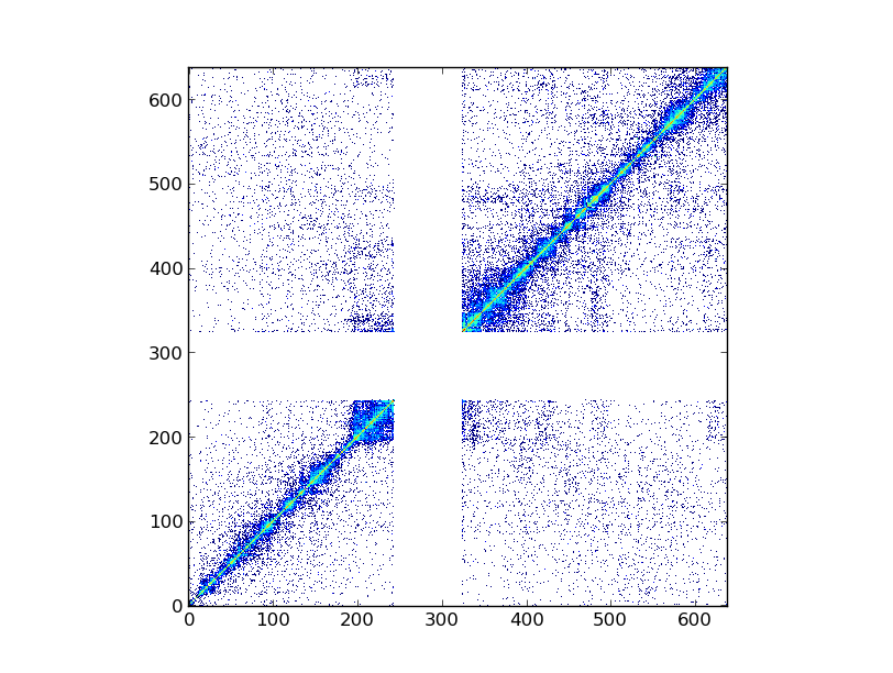
This plot shows the log2 interaction counts, resulting from the given Hi-C experiment.
If the steps in the previous section (Find Topologically Associating Domains) have been done and TADs habe been defined, they can be visualized in the same kind of plot:
my_chrom.visualize("First Hi-C experiment", paint_tads=True, show=True)
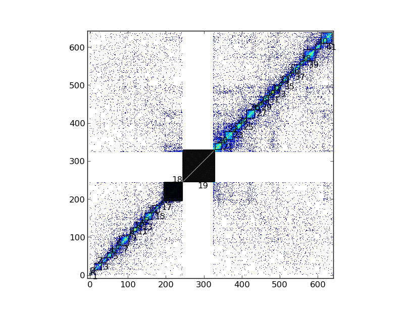
Note: the TAD number 19, corresponding to the centromere, and the TAD number 18, whose size is > 3 Mb, have been shaded
Saving and restoring data
In order to avoid having to calculate TAD positions each time, TADBit allows to save and load Chromosome objects, with all the associated experiments. To save a Chromosome object:
my_chrom.save_chromosome("some_path.tdb")
And to load it:
from pytadbit import load_chromosome

my_chrom = load_chromosome("some_path.tdb")
Note: while information about TADs can be saved, in order to save disk space, raw Hi-C data are not stored in this way but can be loaded again for each experiment:
expr = my_chrom.experiments["First Hi-C experiment"]

expr.load_experiment("sample_data/HIC_k562_chr19_chr19_100000_obs.txt")