Setup¶

The RSmap package requires three other R packages: RCurl (for making http requests with R), bitops (a dependency of RCurl), and RJSONIO (for converting JSON objects retrieved from a sMAP archive into R objects).

The use of RCurl also requires libcurl. If you run into problems installing RCurl, you may need to install it.

To install RSmap, download the package archive and install directly from R, making sure you’re in the correct directory:

> package.install("RSmap_1.0.tar.gz", repos=NULL)

Alternatively you can install the package from the command line:

R CMD install RSmap_1.0.tar.gz

To use the bindings, simply load the library and create a connection:

library(RSmap)
RSmap("http://www.openbms.org/backend")

You can download a working copy of this example, and then follow along with the explanation.

Basic access by UUID¶

Once you’ve got a client, you can start to retrieve data. In the simplest form of access, you already know the UUIDs of the streams you’re interested in. If you have that, you can access directly by range-query. The data retrieval method expects the range to be supplied in the form of Unix timestamps in milliseconds. UTC seconds can be easily generated using strptime, and then converted by multiplication:

start <- as.numeric(strptime("3-29-2013", "%m-%d-%Y"))*1000
end <- as.numeric(strptime("3-31-2013", "%m-%d-%Y"))*1000

oat <- list("395005af-a42c-587f-9c46-860f3061ef0d",
       "9f091650-3973-5abd-b154-cee055714e59",
       "5d8f73d5-0596-5932-b92e-b80f030a3bf7",
       "d64e8d73-f0e9-5927-bbeb-8d45ab927ca5")

data <- RSmap.data_uuid(oat, start, end)

data is returned as an R list of data frames, each element corresponding to a uuid in the oat list. Each entry of the list is a data frame with three properties: time, value, and uuid. For example, the values of the ith entry in data can be accessed with:

data[[i]]$value

The uuid property of course contains the uuid of the stream, while the time property contains the time in UTC milliseconds corresponding to the values.

Plotting this data¶

Plotting the data retrieved with RSmap.data_uuid or other functions can be done after a bit of housekeeping. First, we need to make sure we have the extents of the data so that the series are all visible in the y dimension. This can be set with a simple helper function:

# returns a vector containing the min and max of the data
getExtents <- function(d){
  ex <- lapply(d, function(el){
    c(min(el$value), max(el$value))
  })
  ex <- unlist(ex)
  c(min(ex), max(ex))
}

ylim <- getExtents(data)

Next, we need to be sure we supply UTC seconds to the R date conversion functions when we format the axis:

# convert to UTC seconds for R plot
time_UTC_sec <- data[[1]]$time/1000

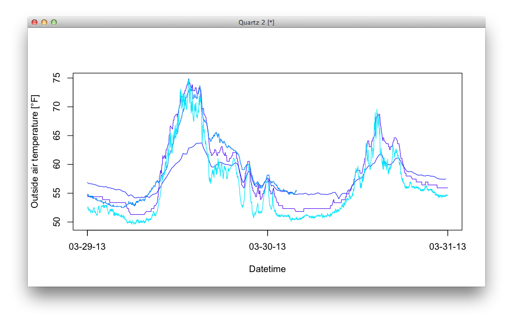
Now we’re ready to set up the plot, format the axis, and draw the series:

# choose some pretty colors
col <- topo.colors(10)

# set up the plot and draw the first series
plot(time_UTC_sec
   , data[[1]]$value
   , xaxt="n"
   , type="l"
   , col=col[1]
   , ylim=ylim
   , xlab="Datetime"
   , ylab="Outside air temperature [°F]")

# format the x-axis to be the local time
axis.POSIXct(side=1, as.POSIXct(time_UTC_sec, origin="1970-01-01"),  format="%m-%d-%y")

# plot the rest of the series
for (i in 2:length(data)){
  lines(data[[i]]$time/1000, data[[i]]$value, col=col[i])
}

Whether the data was retrieved with RSmap.data_uuid, RSmap.next, RSmap.prev, or any of the functions that retrieve time series data, the same technique can be used to plot it.

Access by sMAP Query¶

The archiver also includes a Query Language, which allows SQL-like queries on data metadata. Rather than hard-coding lists of time series UUIDS, you can instead retrieve data on the basis of tags. For instance, we could instead retrieve the weather data in the previous example using a tag query:

data <- RSmap.data("Metadata/Extra/Type = 'oat'", start, end)

The first argument to RSmap.data is a where clause, restricting the set of time series returned to ones with appropriate tags. In this case, we know that the data we’re interested in is tagged with a Metadata/Extra/Type value set to oat.

In order to figure out which feed is which, we might instead want to retrieve the metadata for these streams. We can do this using the RSmap.tags method:

tags <- RSmap.tags("Metadata/Extra/Type = 'oat'")

The metadata is returned as a nested list structure, which you can inspect and match up with returned data using the uuids.

The following example puts this all together by creating a legend for the plot, using data and tags.

In order to explore what tags and values are available, you can try the stream status interface. This lets you explore the set of allowable tags and tag values using a graphical interface, and see some example data. Once you’ve located the data you’re interested in, you can either hard-code the UUIDs or encode that tag query directly into your application.

Additional Library Functionality¶

The client library contains several other methods for accessing data efficiently; for instance, you can get the latest data or access data relative to an reference timestamp.

RSmap(url, key="", private=FALSE, timeout=50.0)

Create a connection to a sMAP archive located at url. The url should point the the root resource of the archive. API keys can be provided as a list, as c(<key1>, <key2>). Set private to TRUE if you only want to get private streams.

RSmap.latest(where, limit=1, streamlimit=10)

Load the last data in a time-series.

See prev for args.

RSmap.prev(where, ref, limit=1, streamlimit=10)

Load data before a reference timestamp. For instance, to locate the last reading whose timestamp is less than the current time, you can use RSmap.prev(where_clause, as.numeric(Sys.time()))

Parameters: where (str) – a selector identifying the streams to query ref (int) – reference timestamp limit (int) – the maximum number of points to retrieve per stream streamlimit (int) – the maximum number of streams to query

Returns: a list of data frames with properties time, value, and uuid containing the data corresponding to one of the uuids from the input.

RSmap.next(where, ref, limit=1, streamlimit=10)

Load data after a reference time.

See prev for args.

RSmap.data(where, start, end, limit=10000)

Load data for streams matching a particular query.

Parameters: where (str) – the ArchiverQuery selector for finding time series start (int) – query start time in UTC seconds (inclusive) end (int) – query end time in UTC seconds (exclusive) Returns: a list of data frames with properties time, value, and uuid containing the data corresponding to one of the uuids from the input.

RSmap.data_uuid(uuids, start, end, cache=True, limit=-1)

Low-level interface for loading a time range of data from a list of uuids.

Parameters: uuids (list) – a list of stringified UUIDs start (int) – the timestamp of the first record in seconds, inclusive end (int) – the timestamp of the last record, exclusive Returns: a list of data frames with properties time, value, and uuid containing the data corresponding to one of the uuids from the input.

RSmap.tags(where)

Load the tags for all streams matching the where clause.

Returns: an R nested list structure containing the metadata of the streams matching the where clause.