Performance and Robustness Testing
Introduction
In developing statistical inference applications, it is essential to test the robustness of one’s software to errors and noise of various kinds. Thus, QInfer provides tools to do so by repeatedly running estimation tasks to measure performance, and by corrupting likelihood calculations in various realistic ways.
Testing Estimation Performance
Given an estimator, a common question of interest is what risk that estimator incurrs; that is, what is the expected error of the estimates reported by the estimator? This is formalized by defining the loss \(L(\hat{\vec{x}}, \vec{x})\) of an estimate \(\hat{\vec{x}}\) given a true value \(\vec{x}\). In QInfer, we adopt the quadratic loss \(L_Q\) as a default, defined as
where \(\matr{Q}\) is a positive-semidefinite matrix that establishes the relative scale of each model parameter.
We can now define the risk for an estimator as
As the risk is defined by an expectation value, we can estimate it by again Monte Carlo sampling over trials. That is, for a given true model \(\vec{x}\), we can draw many different data sets and then find the corresponding estimate for each in order to determine the risk.
Similarly, the Bayes risk \(r(\hat{\vec{x}}(\cdot), \pi)\) is defined by also taking the expectation over a prior distribution \(\pi\),
The Bayes risk can thus be estimated by drawing a new set of true model
parameters with each trial.
QInfer implements risk and Bayes risk estimation by providing
a function perf_test() which simulates a single trial
with a given model, an
experiment design heuristic, and either
a true model parameter vector or a prior distribution. The
perf_test_multiple() function then collects the results
of perf_test() for many trials, reporting an array of
performance metrics that can be used to quickly compute the risk and
Bayes risk.
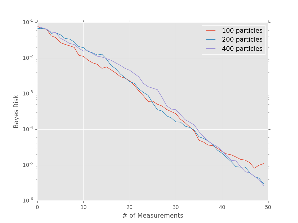
For example, we can use performance testing to evaluate the Bayes
risk as a function of the number of particles used in order to
determine quality parameters in experimental practice. Consider
the simple precession model (SimplePrecessionModel)
under an exponentially sparse sampling heuristic
(ExpSparseHeuristic). Then, we can test the performance
of estimating the precession frequency for several different
values of n_particles:
model = SimplePrecessionModel()
prior = UniformDistribution([0, 1])
heuristic_class = ExpSparseHeuristic

for n_particles in [100, 200, 400]:
    perf = perf_test_multiple(
        n_trials=50,
        model=model, n_particles=n_particles, prior=prior,
        n_exp=50, heuristic_class=heuristic_class
    )
    # The array returned by perf_test_multiple has
    # shape (n_trials, n_exp), so to take the mean over
    # trials (Bayes risk), we need to average over the
    # zeroth axis.
    bayes_risk = perf['loss'].mean(axis=0)

    plt.semilogy(bayes_risk, label='{} particles'.format(n_particles))

plt.xlabel('# of Measurements')
plt.ylabel('Bayes Risk')
plt.legend()
plt.show()
(Source code, svg, pdf, hires.png, png)

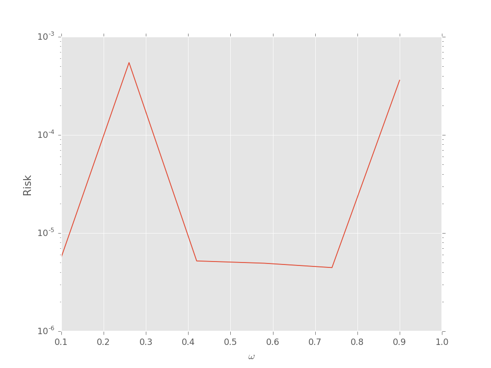
We can also pass fixed model parameter vectors to evaluate the risk (that is, not the Bayes risk) as a function of the true model:
model = SimplePrecessionModel()
prior = UniformDistribution([0, 1])
heuristic_class = ExpSparseHeuristic
n_exp = 50

omegas = np.linspace(0.1, 0.9, 6)
risks = np.empty_like(omegas)

for idx_omega, omega in enumerate(omegas[:, np.newaxis]):
    perf = perf_test_multiple(
        n_trials=100,
        model=model, n_particles=400, prior=prior,
        n_exp=n_exp, heuristic_class=heuristic_class,
        true_mps=omega
    )
    # We now only take the loss after the last
    # measurement (indexed by -1 along axis 1).
    risks[idx_omega] = perf['loss'][:, -1].mean(axis=0)

plt.semilogy(omegas, risks)

plt.xlabel(r'$\omega$')
plt.ylabel('Risk')
plt.show()
(Source code, svg, pdf, hires.png, png)

Robustness Testing
Incorrect Priors and Models
The perf_test() and perf_test_multiple()
functions also allow for testing the effect of “bad” prior
assumptions, and of using the “wrong” model for estimation.
In particular, the true_prior and true_model arguments
allow for testing the effect of using a different prior or
model for performing estimation than for simulating data.
Modeling Faulty or Noisy Simulators
In addition, QInfer allows for testing robustness
against errors in the model itself by using
PoisonedModel.
This derived model
adds noise to a model’s likelihood()
method in such a way as to simulate sampling errors incurred in
likelihood-hood free parameter estimation (LFPE) approaches
[FG13]. The noise that PoisonedModel adds can be specified as the
tolerance of an adaptive likelihood estimation (ALE) step [FG13], or as the number
of samples and hedging used for a hedged maximum likelihood estimator of
the likelihood [FB12]. In either case, the requested noise is added to the
likelihood reported by the underlying model, such that
where \(\widehat{\Pr}\) is the reported estimate of the true likelihood.
For example, to simulate using adaptive likelihood estimation to reach a threshold tolerance of 0.01:
>>> from qinfer import SimplePrecessionModel, PoisonedModel
>>> model = PoisonedModel(SimplePrecessionModel(), tol=0.01)
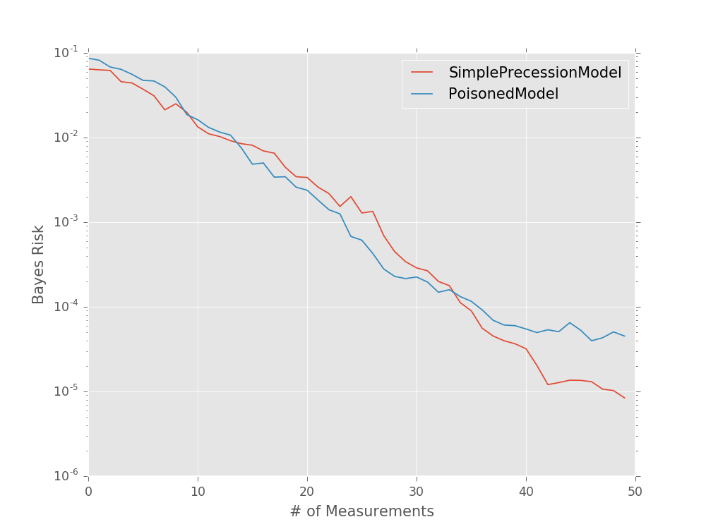
We can then use perf_test_multiple() as above to
quickly test the effect of noise in the likelihood function on
the Bayes risk.
models = [
    SimplePrecessionModel(),
    PoisonedModel(SimplePrecessionModel(), tol=0.25)
]
prior = UniformDistribution([0, 1])
heuristic_class = ExpSparseHeuristic

for model in models:
    perf = perf_test_multiple(
        n_trials=50,
        model=model, n_particles=400, prior=prior,
        true_model=models[0],
        n_exp=50, heuristic_class=heuristic_class
    )
    bayes_risk = perf['loss'].mean(axis=0)

    plt.semilogy(bayes_risk, label=type(model).__name__)

plt.xlabel('# of Measurements')
plt.ylabel('Bayes Risk')
plt.legend()
plt.show()
(Source code, svg, pdf, hires.png, png)
