pymodelfit.builtins.LinearModel
- class pymodelfit.builtins.LinearModel[source]
Bases: pymodelfit.core.FunctionModel1DAuto
 linear model.
A number of different fitting options are available - the fittype attribute determines which type should be used on calls to fitData. It can be:
- ‘basic’
Analytically compute the parameters from simple least-squares form. If weights are provided they will be interpreted as
 or
or 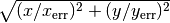 if a
2-tuple.
if a
2-tuple.
- ‘yerr’:
Same as weighted version of basic, but weights are interpreted as y-error instead of inverse.
- ‘fiterrxy’:
Allows errors in both x and y using the chi^2 from the fitexy algorithm from numerical recipes. weights must be a 2-tuple (xerr,yerr).
- __init__()
x.__init__(...) initializes x; see help(type(x)) for signature
Methods
chi2Data([x, y, weights, ddof]) Computes the chi-squared statistic for the data assuming this model. derivative(x[, dx]) distanceToPoint(xp, yp) Computes the shortest distance from this line to a provided point or points. f(x[, m, b]) findroot(x0[, method]) Finds a root for the model (location where the model is 0). findval(val, x0[, method]) Finds where the model is equal to a specified value. fitBasic(x, y[, fixslope, fixint]) Does the traditional fit based on simple least-squares regression for a linear model  .
.fitData([x, y, fixedpars, weights, ...]) Fit the provided data using algorithms from scipy.optimize, and adjust the model parameters to match. fitErrxy(x, y, xerr, yerr, **kwargs) Uses the chi^2 statistic .. fitWeighted(x, y[, sigmay, doplot, ...]) Does a linear weighted least squares fit and computes the coefficients and errors. fromPowerLaw(plmod[, base]) Takes a PowerLawModel and converts it to a linear model assuming getCall() Retreives infromation about the calling function. getCov() Computes the covariance matrix for the last fitData() call. getMCMC(x, y[, priors, datamodel]) Generate an Markov Chain Monte Carlo sampler for the data and model. integrate(lower, upper[, method]) integrateCircular(lower, upper, *args, **kwargs) Integrate this model on the 2D circle. This calls integrate() with integrateSpherical(lower, upper, *args, **kwargs) Integrate this model on the 3D sphere. This calls integrate() with inv(yval, *args, **kwargs) Find the x value matching the requested y-value. isVarnumModel() Determines if the model represented by this class accepts a variable number of parameters (i.e. maximize(x0[, method]) Finds a local maximum for the model. minimize(x0[, method]) Finds a local minimum for the model. pixelize(xorxl[, xu, n, edge, sampling]) Generate a discretized version o the model. plot([lower, upper, n, clf, logplot, data, ...]) Plot the model function and possibly data and error bars with matplotlib.pyplot. plotResiduals([x, y, clf, logplot]) Plots the residuals of the provided data (  ) against this model.
pointSlope(m, x0, y0) Sets model parameters for the given slope that passes through the point. resampleFit([x, y, xerr, yerr, bootstrap, ...]) Estimates errors via resampling. residuals([x, y, retdata]) Compute residuals of the provided data against the model. setCall([calltype, xtrans, ytrans]) Sets the type of function evaluation to occur when the model is called. stdData([x, y]) Determines the standard deviation of the model from data. twoPoint(x0, y0, x1, y1) Sets model parameters to pass through two lines (identical behavior Attributes
b int(x=0) -> int or long data The fitting data for this model. defaultIntMethod str(object=’‘) -> string defaultInvMethod str(object=’‘) -> string defaultparval int(x=0) -> int or long errors Error on the data. fittype str(object=’‘) -> string fittypes A Sequence of the available valid values for the fittype fixedpars tuple() -> empty tuple m int(x=0) -> int or long params A tuple of the parameter names. pardict A dictionary mapping parameter names to the associated values. parvals The values of the parameters in the same order as params rangehint weightstype Determines the statistical interpretation of the weights in data. xaxisname yaxisname - chi2Data(x=None, y=None, weights=None, ddof=1)
Computes the chi-squared statistic for the data assuming this model.
Parameters: - x (array-like or None) – Input data value or None to use stored data
- y (array-like or None) – Output data value or None to use stored data
- weights (array-like or None) – Weights to adjust chi-squared, typically for error bars. Statistically interpreted based on the weightstype attribute. If None, any stored data will be used.
- ddof (int) – Delta Degrees of Freedom. The divisor used for the reduced chi-squared is n-m-ddof, where N is the number of points and m is the number of parameters in the model.
Returns: tuple of floats (chi2,reducedchi2,p-value)
- data None
The fitting data for this model. Should be either None, or a tuple(datain,dataout,weights). Note that the weights are interpreted statistically as errors based on the weightstype attribute.
- distanceToPoint(xp, yp)[source]
Computes the shortest distance from this line to a provided point or points.
The distance is signed in the sense that a positive distance indicates the point is above the line (y_point>y_model) while negative is below.
Parameters: - xp (scalar or array-like) – The x-coordinate of the point(s).
- yp (scalar or array-like) – The y-coordinate of the point(s). Length must match xp.
Returns: The (signed) shortest distance from this model to the point(s). If xp and yp are scalars, this will be a scalar. Otherwise, it is an array of shape matching xp and yp.
- errors None
Error on the data. Sets the weights on data assuming the interpretation for errors given by weightstype. If data is None/missing, a TypeError will be raised.
- findroot(x0, method='fmin', **kwargs)
Finds a root for the model (location where the model is 0).
Parameters: kwargs are passed into the method function
Returns: the x value where the model is 0
- findval(val, x0, method='fmin', **kwargs)
Finds where the model is equal to a specified value.
x0 is the location to start the search method can be ‘fmin’ or ‘fmin_powell’ (from scipy.optimize) kwargs are passed into the scipy.optimize function
- static fitBasic(x, y, fixslope=False, fixint=False)[source]
Does the traditional fit based on simple least-squares regression for a linear model
.Parameters: - x (array-like) – x data for the fit
- y (array-like) – y data for the fit
- fixslope (scalar or False or None) – If False or None, the best-fit slope will be found. Otherwise,specifies the value to assume for the slope.
- fixint (scalar or False or None) – If False or None, the best-fit intercept will be found. Otherwise,specifies the value to assume for the intercept.
Returns: ((m,b)),dm,db,dy)
- fitData(x=None, y=None, fixedpars='auto', weights=None, savedata=True, updatepars=True, fitf=False, contraction='sumsq', **kwargs)
Fit the provided data using algorithms from scipy.optimize, and adjust the model parameters to match.
The fitting technique is sepcified by the fittype attribute of the object, which by default can be any of the optimization types in the scipy.optimize module (except for scalar minimizers)
The full fitting output is available in lastfit attribute after this method completes.
Parameters: - x (array-like) – The input values at which to evaluate the model. Valid shapes are those that this model will accept.
- y (array-like) – The expected output values for the model at the given x values. Valid shapes are those that this model will output.
- fixedpars (sequence of strings, ‘auto’ or None) – Parameter names to leave fixed. If ‘auto’ the fixed parameters are inferred from self.fixedpars (or all will be free parameters if self.fixedpars is absent). If None, all parameters will be free.
- weights –
Weights to use for fitting, statistically interpreted as inverse errors (not inverse variance). May be one of the following forms:
- None for equal weights
- an array of points that must match the output
- a 2-sequence of arrays (xierr,yierr) such that xierr matches the x-data and yierr matches the y-data
- a function called as f(params) that returns an array of weights that match one of the above two conditions
- savedata (bool) – If True, x,`y`,and weights will be saved to data. Otherwise, data will be discarded after fitting.
- updatepars (bool) – If True, sets the parameters on the object to the best-fit values.
- fitf (bool) – If True, the fit is performed directly against the f() method instead of against the model as evaluated if called (as altered using setCall()).
- contraction –
Only applies for optimize-based methods and is the technique used to convert vectors to figures of merit. this is composed of multiple string segments:
- these will be applied to each element of the vector first:
- ‘sq’: square
- ‘abs’:absolute value
- ‘’:raw value
- the contraction is performed after:
- ‘sum’: sum of all the elements
- ‘median’: median of all the elements
- ‘mean’: mean of all the elements
- ‘prod’: product of all the elements
- optionally,the string can include ‘frac’ to use the fractional version of the differnce vector instead of raw values. For the leastsq method, this is the only applicable value
- these will be applied to each element of the vector first:
kwargs are passed into the fitting function.
Returns: array of the best fit parameters Raises ModelTypeError: If the output of the model does not match the shape of y. See also
- fitErrxy(x, y, xerr, yerr, **kwargs)[source]
Uses the chi^2 statistic
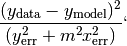
to fit the data with errors in both x and y.
Parameters: - x (array-like) – x data for the fit
- y (array-like) – y data for the fit
- xerr (array-like) – Error/standard deviation on x.
- yerr (array-like) – Error/standard deviation on y.
kwargs are passed into scipy.optimize.leastsq
Returns: best-fit (m,b) Note
Fitting results are saved to lastfit
- static fitWeighted(x, y, sigmay=None, doplot=False, fixslope=None, fixint=None)[source]
Does a linear weighted least squares fit and computes the coefficients and errors.
Parameters: - x (array-like) – x data for the fit
- y (array-like) – y data for the fit
- sigmay (array-like or None) – Error/standard deviation on y. If None, weights are equal.
- fixslope (scalar or None) – The value to force the slope to or None to leave the slope free.
- fixint (scalar or None) – The value to force the intercept to or None to leave intercept free.
Returns: tuple (m,b,sigma_m,sigma_b)
- fittypes None
A Sequence of the available valid values for the fittype attribute. (Read-only)
- static fromPowerLaw(plmod, base=10)[source]
Takes a PowerLawModel and converts it to a linear model assuming ylinear = log_base(ypowerlaw) and xlinear = log_base(xpowerlaw)
returns the new LinearModel instance
- getCall()
Retreives infromation about the calling function.
Returns: The type of evaluation to perform when this model is called - a string like that of the type passed into setCall(), or None if the model function itself is to be called.
- getCov()
Computes the covariance matrix for the last fitData() call.
Returns: The covariance matrix with variables in the same order as params. Diagonal entries give the variance in each parameter. Warning
This is not guaranteed to work for custom fit-types, but will always work with the default (leastsq) fit.
- getMCMC(x, y, priors={}, datamodel=None)
Generate an Markov Chain Monte Carlo sampler for the data and model. This function requires the PyMC package for the MCMC internals and sampling.
Parameters: - x (array-like) – Input data value
- y (array-like) – Output data value
- priors (dictionary) –
Maps parameter names to the priors to assume for that parameter. There must be an entry for every parameter in the model. The prior specification can be in any of the following forms:
- A pymc.Stochastric object
- A 2-tuple (lower,upper) for a uniform prior
- A scalar > 0 to use a gaussian prior of the provided width centered at the current value of the parameter
- 0 for a Poisson prior with k set by the current value of the parameter
- datamodel –
Specifies the model to assume for the fitting data points. May be any of the following:
- None
- A normal distribution with sigma given by the data’s standard deviation.
- A tuple (dist,dataname,kwargs)
- The first element is the pymc.distribution to be used as the distribution representing the data and the second is the name of the argument to be associated with the FunctionModel1D’s output, and the third is kwargs for the distribution (“observed” and “data” will be ignored, as will the data argument)
- A sequence
- A normal distribution is used with sigma for each data point specified by the sequence. The length must match the model.
- A scalar
- A normal distribution with the given standard deviation.
Raises ValueError: If a prior is not provided for any parameter.
Returns: A pymc.MCMC object ready to sample for this model.
- integrateCircular(lower, upper, *args, **kwargs)
Integrate this model on the 2D circle. This calls integrate() with the jacobian set appropriately assuming the model is the radial profile for an azimuthally symmetric 2D surface density.
If a jac keyword is provided, it is taken as an additional factor to multiply the circular jacobian.
- integrateSpherical(lower, upper, *args, **kwargs)
Integrate this model on the 3D sphere. This calls integrate() with the jacobian set appropriately assuming the model is the radial profile for a spherically symmetric 3D density.
If a jac keyword is provided, it is taken as an additional factor to multiply the circular jacobian.
- inv(yval, *args, **kwargs)
Find the x value matching the requested y-value. The inverse is computed using root finders from the scipy.optimize module.
Parameters: yval (float) – the output y-value at which to compute the inverse Other args and kwargs are those appropriate for the chosen root-finder, except for the keyword method which can be a name of any of the root finders from scipy.optimize. method can also be a function that should take f(g(x),*args,**kwargs) and return the x value at which g(x) is 0.
The default method depends on the input arguments as follows:
- inv(yval)
- inv(yval,x0)
Uses scipy.optimize.newton(), starting the search at x0
- inv(yval,a,b)
Uses scipy.optimize.brentq(), searching the bracketing interval [a,b] for the lower and upper edges of the search range.
Returns: the x-value at which the model equals the given yval Examples
This finds the x value of the (very simple) function
 at the point y=3
>>> from pymodelfit.builtins import LinearModel
>>> m = LinearModel(m=4,b=2)
>>> '%.2f'%m.inv(3)
'0.25'
These examples use Newton’s, Brent’s, and Ridder’s method, to find the inverse of :math`y(x) = x^2` for 2,9,and 16, respectively (i.e. they should give sqrt(2),3, and 4)
>>> from pymodelfit.builtins import QuadraticModel
>>> m = QuadraticModel()
>>> '%.2f'%m.inv(2,1)
'1.41'
>>> '%.2f'%m.inv(9,2,4)
'3.00'
>>> '%.2f'%m.inv(16,3,5,method='ridder')
'4.00'
All these methods require a guide for the range of x values to search. The first requires a guess, although the default guess of 0 will be assumed if the second argument is not present. (for this example, sqrt(2) and -sqrt(2) are both valid answers, so the default guess of 0 is ambiguous).
- classmethod isVarnumModel()
Determines if the model represented by this class accepts a variable number of parameters (i.e. number of parameters is set when the object is created).
Returns: True if this model has a variable number of parameters.
- maximize(x0, method='fmin', **kwargs)
Finds a local maximum for the model.
Parameters: kwargs are passed into the method function
Returns: a x value where the model is a local maximum
- minimize(x0, method='fmin', **kwargs)
Finds a local minimum for the model.
Parameters: kwargs are passed into the method function
Returns: a x value where the model is a local minimum
- params None
A tuple of the parameter names. (read-only)
- pardict None
A dictionary mapping parameter names to the associated values.
- pixelize(xorxl, xu=None, n=None, edge=False, sampling=None)
Generate a discretized version o the model. This method integrates over the model for a number of ranges to get a 1D “pixelized” version of the model.
Parameters: - xoroxl – If array, specifies the location of each of the pixels. If float, specifies the lower edge of the pixelized section.
- xu (float) – Specifies the upper edge of the pixelized section. Ignored if xorxl is array-like.
- n (int) – Specifies the number of pixels. Ignored if xorxl is array-like.
- edge (bool) – If True, pixel locations are for the edges (xorxl lower edges, xu upper edge), or if False, they are pixel centers.
- sampling (int or None) – If None, each pixel will be computed by integrating. Otherwise, the number of samples to use in each pixel.
Returns: Integrated values for the function as an array of size n or matching xorxl.
- plot(lower=None, upper=None, n=100, clf=True, logplot='', data='auto', errorbars=True, *args, **kwargs)
Plot the model function and possibly data and error bars with matplotlib.pyplot. The plot will reflect any changes applied with setCall().
Parameters: - lower (scalar or None) – The starting x value for the plot. If None, the bound will be inferred from the data argument to this function or the rangehint attribute of the model.
- upper (scalar or None) – The ending x value for the plot. If None, the bound will be inferred from the data argument to this function or the rangehint attribute of the model.
- n (int) – The number of samples for the plot
- clf (boolean) – If True, the figure will be cleared before the plot is drawn.
- logplot (‘’,’x’,’y’, or ‘xy’ string) – Sets which axes are logarithmic
- data (‘auto’, None, or array like of the form (x,y) or (x,y,(xerr,yerr))) – Determines what (if any) data to display. If None, no data is displayed. If ‘auto’, data from the data attribute of the FunctionModel1D will be used if present, or nothing if the data attribute is empty or None. Otherwise, the data to be plotted (and possibly errors) can be provided as arrays. Or if a dictionary is given, it will be treated as keyword arguments to the matplotlib.pyplot.scatter() function (possibly with data as ‘xdata’,’ydata’,and ‘weights’ entries).
- errorbars (boolean) – If True and weights are present in the data, error bars are shown on the data based on the interpretation given by the weightstype attribute. If False, no error bars are shown.
Additional arguments and keywords are passed into matplotlib.pyplot.plot().
Note
By default, the model is plotted over the data points. If the points should be drawn on top of the model, set the keyword argument zorder to 0.
- plotResiduals(x=None, y=None, clf=True, logplot='', **kwargs)
Plots the residuals of the provided data (
) against this
model.Parameters: - x (array-like or None) – The x data to plot the residuals for, or None to get it from any fitted data.
- y (array-like or None) – The x data to plot the residuals for, or None to get it from any fitted data.
- clf (bool) – If True, the plot will be cleared first.
- logplot (‘’,’x’,’y’, or ‘xy’ string) – Sets which axes are logarithmic
Additional arguments and keywords are passed into matplotlib.pyplot.scatter().
- pointSlope(m, x0, y0)[source]
Sets model parameters for the given slope that passes through the point.
Parameters:
- resampleFit(x=None, y=None, xerr=None, yerr=None, bootstrap=False, modely=False, n=250, prefit=True, medianpars=False, plothist=False, **kwargs)
Estimates errors via resampling. Uses the fitData function to fit the function many times while either using the “bootstrap” technique (resampling w/replacement), monte carlo estimates for the error, or both to estimate the error in the fit.
Parameters: - x (array-like or None) – The input data - if None, will be taken from the data attribute.
- y (array-like or None) – The output data - if None, will be taken from the data attribute.
- xerr (array-like, callable, or None) – Errors for the input data (assumed to be normally distributed), or if None, will be taken from the data. Alternatively, it can be a function that accepts the input data as the first argument and returns corresponding monte carlo sampled values.
- yerr (array-like, callable, or None) – Errors for the output data (assumed to be normally distributed), or if None, will be taken from the data. Alternatively, it can be a function that accepts the output data as the first argument and returns corresponding monte carlo sampled values.
- bootstrap (bool) – If True, the data is also resampled (with replacement).
- modely – If True, the fitting data will be generated by offseting from model values (evaluated at the x-values) instead of y-values.
- n (int) – The number of times to draw samples.
- prefit (bool) – If True, the data will be fit without resampling once before the samples are recorded.
- medianpars (bool) – If True, the median from the histogram will be set as the value for the parameter.
- plothist (bool or string) – If True, histograms will be plotted using matplotlib.pyplot.hist() for each of the parameters, or if it is a string, only the histogram for the requested parameter will be shown.
kwargs are passed into fitData
Returns: (histd,cov) where histd is a dictionary mapping parameters to their histograms and cov is the covariance matrix of the parameters in parameter order. Note
If x, y, xerr, or yerr are provided, they do not overwrite the stored data, unlike most other methods for this class.
- residuals(x=None, y=None, retdata=False)
Compute residuals of the provided data against the model. E.g.
 .
.Parameters: Returns: Residuals of model from y or if retdata is True, a tuple (x,y,residuals).
Return type: array-like
- setCall(calltype=None, xtrans=None, ytrans=None, **kwargs)
Sets the type of function evaluation to occur when the model is called. Changes the output of a function call to be
 ,
where
,
where  is set by calltype,
  is given by the
xtrans argument, and
is given by the
xtrans argument, and  is given by ytrans.
Parameters: - calltype –
Specifies what should be output when the model is called. Can be:
- None
- basic function evaluation
- ‘derivative’
- derivative at the location (see derivative())
- ‘integrate’
- integral - specify upper or lower kwargs and the evaluation location will be treated as the other bound. If neither is given, lower = 0 is assumed. (see integrate())
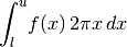
- ‘integrateCircular’
- Polar integration – see integrateCircular()
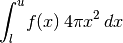
- ‘integrateSpherical’
- Spherical integration – see integrateSpherical()
- Any other string that is the name of a method on this object. It will be called with the function value as its first argument.
- xtrans (string or None) – Transformations applied to the input value before being passed into the model. See below for valid forms.
- ytrans (string or None) – Transformations applied to the output value. See below for valid forms.
Any kwargs are passed into the function specified in calltype.
xtrans and ytrans transformation functions can accept the following values:
- None

- ‘log’
- ‘ln’

- ‘log##.#’
- ‘pow’

- ‘exp’

- ‘pow##.#’
Warning
There may be unintended consequences of this method due to methods using the call value instead of the default function evaluation result. You have been warned...
- calltype –
- stdData(x=None, y=None)
Determines the standard deviation of the model from data. Data can either be provided or (by default) will be taken from the stored data.
Parameters: Returns: standard deviation of model from y
- twoPoint(x0, y0, x1, y1)[source]
Sets model parameters to pass through two lines (identical behavior in fitData).
Parameters:
- weightstype None
Determines the statistical interpretation of the weights in data. Can be:
- ‘ierror’
Weights act as inverse errors (default)
- ‘ivar’
Weights act as inverse variance
- ‘error’
Weights act as errors (non-standard - this makes points with larger error bars count more towards the fit).
- ‘var’
Weights act as variance (non-standard - this makes points with larger error bars count more towards the fit).