Application Example of GP regression

This Example shows the Squared Exponential CF (covar.se.SEARDCF) combined with noise covar.noise.NoiseISOCF by summing them up (using covar.combinators.SumCF).

First of all we have to import all important packages:

import pylab as PL
import scipy as SP
import numpy.random as random

Now import the Covariance Functions and Combinators:

from pygp.covar import se, noise, combinators

And additionally the GP regression framework (pygp.gp and pygp.priors for the priors):

from pygp.gp.basic_gp import GP
from pygp.optimize.optimize import opt_hyper
from pygp.priors import lnpriors
import pygp.plot.gpr_plot as gpr_plot

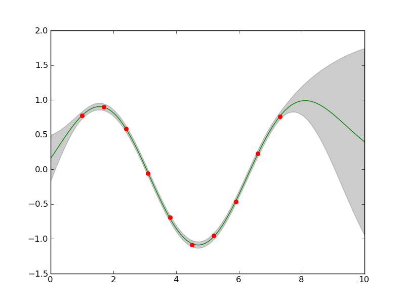
For this particular example we generate some simulated random sinus data, just samples from a superposition of a sin + linear trend:

random.seed(1)
xmin = 1
xmax = 2.5*SP.pi
x = SP.arange(xmin,xmax,0.7)

C = 2       #offset
b = 0.5
sigma = 0.01

b = 0

y  = b*x + C + 1*SP.sin(x)
dy = b   +     1*SP.cos(x)
y += sigma*random.randn(y.shape[0])

y-= y.mean()

x = x[:,SP.newaxis]

The predictions we will make on the interpolation interval

X = SP.linspace(0,10,100)[:,SP.newaxis]

Our starting hyperparameters are:

dim = 1
logthetaCOVAR = SP.log([1,1,sigma])
hyperparams = {'covar':logthetaCOVAR}

Now the interesting point: creating the sumCF by combining noise and se:

SECF = se.SEARDCF(dim)
noiseCF = noise.NoiseISOCF()
covar = combinators.SumCF((SECF,noiseCF))

And the prior believes, we have about the hyperparameters:

#Length-Scale
covar_priors = []
covar_priors.append([lnpriors.lngammapdf,[1,2]])
for i in range(dim):
    covar_priors.append([lnpriors.lngammapdf,[1,1]])
#Noise
covar_priors.append([lnpriors.lngammapdf,[1,1]])
priors = {'covar':covar_priors}

We do want all hyperparameter to be optimized:

Ifilter = {'covar': SP.array([1,1,1],dtype='int')}

Create the GP regression class for further usage:

gpr = GP(covar,x=x,y=y)

And optimize the hyperparameters:

[opt_model_params,opt_lml]= opt_hyper(gpr,hyperparams,priors=priors,gradcheck=False,Ifilter=Ifilter)

With these optimized hyperparameters we can now predict the point-wise mean and deviance of the training data:

[M,S] = gpr.predict(opt_model_params,X)

For the sake of beauty plot the mean and deviance:

gpr_plot.plot_sausage(X,M,SP.sqrt(S))
gpr_plot.plot_training_data(x,y)

The resulting plot is: