This part of TeraPy documentation is dedicated to users, whose main goal is measurement. It concentrates on TeraPy graphical user interface.
Contents
TeraPy can be run in a number of different ways:
import wx
from terapy import TeraPyMainFrame
app = wx.App(redirect=False)
frame = TeraPyMainFrame()
frame.Show(True)
app.MainLoop()
At this point, the main interface should appear and widgets associated with the devices described in devices.ini should be displayed at the bottom of the central panel. If the interface doesn’t show or for any other problem, see the Troubleshooting section.
An overview of the main TeraPy window is found below (TeraPy main window). The interface is divided into distinct sections, which are described in details below.
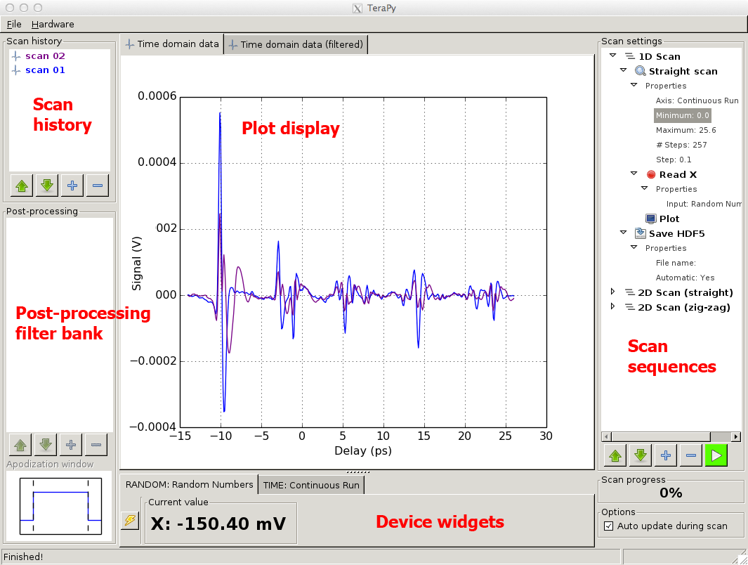
TeraPy main window
TeraPy handles physical units. Devices can provide informations about the units they measure. These will be remembered throughout the post-processing chain.
Units can be either set globally through the Default units menu (see Menus for details), or locally depending on the plot canvas used.
Physical units are managed with the Pint package.
The Scan settings control allows to define scan sequences. A scan sequence ( icon) is presented as a list of scan events.
Scan events can be added to sequences and to events that support children (for example loops). A scan sequence will run only if a measurement event is present. Also, some events, which require measured data (such as save or plot events), can’t run before the data has been measured. Before running a sequence, TeraPy will check these rules for you and issue a warning if necessary. One data container and one history entry will be created for each measurement event present in the sequence.
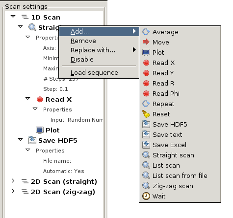
Scan settings with open popup menu
Scan events are added to the tree either with the  button, or through the right-click popup menu (see Scan settings with open popup menu). The additional functions accessible through this menu are
 button) events). Same effect as
  button
Events can be re-organized with the 
 buttons or by drag and drop.
Scan events are configured either by double-clicking on their tree entry or by changing the properties in the Properties folder shown under the event tree entry.
Clicking will run the sequence, which contains the selected event. During measurement, the button turns red and displays  . Click it to stop the ongoing measurement.
The Scan history shows a list of data containers in memory. The adjacent icon gives the data dimension
New entries can be added either by a measurement sequence or by loading from a file. Entries in bold letters are displayed in one plot canvas. Entries are shown/hidden by double-clicking on their name in the list. Plots are added to the 1st available canvas (if none is found, a new canvas is created). If possible, entries are colored like their associated plot. Several actions are available through right-click (see Scan history with open popup menu)
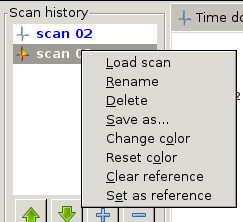
Scan history with open popup menu
Scan data can be displayed in plot canvases. Upon display request, TeraPy will search for an appropriate canvas. If one is found, a plot will be added. Otherwise, TeraPy adds one canvas from the list of available canvas modules, then add a plot to it. Currently, 1D and 2D data are supported.
Plot canvases are either data canvases or post-processing canvases. Data canvases can only display raw, non-processed, data. A Post-processing canvas can be linked with a data canvas or another post-processing canvas (nested post-processing). Commands and options are available by right-click on the canvas tab (see Plot canvas tab with open popup menu), and are
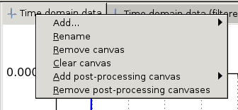
Plot canvas tab with open popup menu
1D data canvases support zooming by click and drag. Simply select the area, which you want to zoom on. Right click restores canvas to original state. In addition, right click on 1D post-processing canvases switches between linear and logarithmic scales.
Post-processing filters are only available if a post-processing canvas is displayed. If so, the post-processing filter control is enabled. The displayed list of filters corresponds to the currently visible plot canvas. A preview of apodization filters is displayed at the bottom of the control. Apodization filters are windowing functions that are applied in view of a domain transform (e.g. Fourier transform). Internally, these filters have the is_pre_filter property set to True (see programmer’s guide Post-processing filters section for details).
Post-processing filters can be added with the button, removed with , and re-arranged with or by drag and drop. Right-clicking on an item shows a popup menu with additional options (see Post-processing filter list with open popup menu):
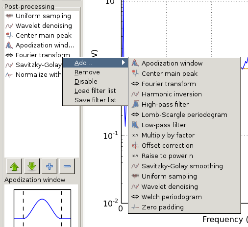
Post-processing filter list with open popup menu
Device drivers can (optionally) provide one or several widgets, which will be added to the device widgets area. Widgets are meant to display instantaneous informations on the device or allow control of some device parameters. Additional informations may be found in the Device drivers section.
Device widgets aren’t accessible while a measurement sequence is running. Device parameters, which you want to set dynamically during measurement, must be treated by a scan event.