Gaussian Process Regression

A simulation is seen as a function \(f(x)+\epsilon\) (\(x \in \mathbb{R}^D\)) with additional random error \(\epsilon \sim \mathcal{N}(0,v_t)\). This optional error is due to the stochastic nature of most simulations.

Note

This error does not depend on \(x\). An extension to model an error depending on \(x\) will be added in the future.

The GaussianProcess module uses regression to model the simulation as a Gaussian process. We refer to Girard’s thesis [1] for a really good explanation of GP regression.

“A Gaussian process is a collection of random variables, any finite number of which have (consistent) joint Gaussian distributions.” – Rasmussen, C. E. Gaussian Processes in Machine Learning, Advanced Lectures on Machine Learning, Springer Berlin Heidelberg, 2004, 3176, 63-71

“Once the mean and covariance functions are defined, everything else about GPs follows from the basic rules of probability applied to multivariate Gaussians.” – Zoubin Ghahramani

Note

The following explanation is an excerpt from my paper [2].

\(m(x) = E[G(x)]\) (\(x\in\mathbb{R}^d\)) is the mean function of the Gaussian process and \(C(x_i,x_j) = \mathrm{Cov}[G(x_i),G(x_j)]\) is the covariance function. For any given set of inputs \(\{x_1,\dots,x_n\}\), \((G(x_1),\dots,G(x_n))\) is a random vector with an \(n\)-dimensional normal distribution \(\mathcal{N}({\mu},\Sigma)\). \({\mu}\) is the vector of mean values \((m(x_1),\dots,m(x_n))\) and \(\Sigma\) is the covariance matrix with \(\Sigma_{ij} = C(x_i,x_j)\)

For modeling \(f(x)\), we use the Gaussian squared exponential covariance function \(C(x_i,x_j) = v \exp \left[-\tfrac{1}{2}(x_i-x_j)^T {W}^{-1}(x_i-x_j)\right]\), as it performs well regarding accuracy. Without loss of generality, we use \(m(x)=m\).

\({W}^{-1} = \mathrm{diag}(w_1,\dots,w_d)\) and \(v\) are hyperparameters of the Gaussian process. We have a set of observed simulation results \(\mathcal{B} = \{(x_i,t_i)\}_{i=1}^N\) as supporting points with \(x_i \in \mathbb{R}^d\) and \(t_i = f(x_i)+\epsilon_i\) with white noise \(\epsilon_i \sim \mathcal{N}(0,v_t)\). This noise represents the aleatory uncertainty of the simulation that calculates \(f(x)\).

To model the noisy observations \(t_i\) we use \(K=\Sigma + v_t I\) as covariance matrix for regression. Therefore, we have an additional hyperparameter \(v_t\). The hyperparameters \(W^{-1}\), \(v_t\), and \(v\) can be estimated from a given dataset with a maximum likelihood approach. In the following, we use \({\beta}={K}^{-1}{t}\) with \({t} = (t_1,\dots,t_N)^T\) to simplify notation.

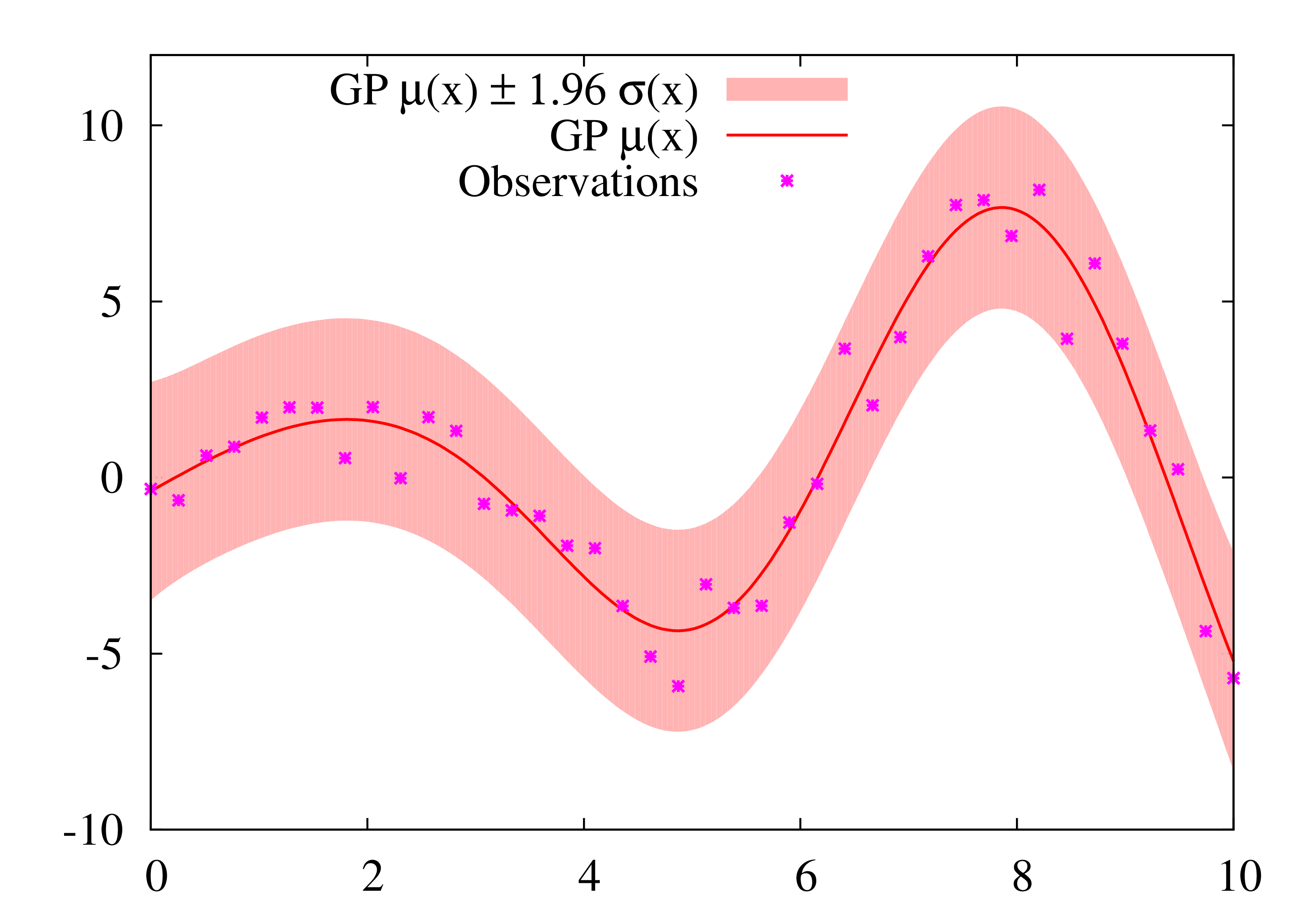
Now, the Gaussian process can be used as a surrogate for the simulation model. The prediction \(\mu(x)\) and code plus aleatory uncertainty \(\sigma^2 (x)\) at a new input \(x\) is:

\[\begin{split}\mu (x) &= \sum_{i=1}^N \beta_i C(x,x_i) \\ \sigma^2 (x) &= C(x,x) - \sum_{i,j=1}^N K_{ij}^{-1}C(x,x_i)C(x,x_j) + v_t\end{split}\]

1-d Example:

Usage: See Getting Started

References

[1]	Girard, A. Approximate Methods for Propagation of Uncertainty with Gaussian Process Models, University of Glasgow, 2004

[2]	Baumgaertel, P.; Endler, G.; Wahl, A. M. & Lenz, R. Inverse Uncertainty Propagation for Demand Driven Data Acquisition, Proceedings of the 2014 Winter Simulation Conference, IEEE Press, 2014, 710-721 (https://www6.cs.fau.de/publications/public/2014/WinterSim2014_baumgaertel.pdf)