scikit-fmm documentation
scikit-fmm is a python extension module which implements the
fast marching method.
The fast marching method is used to model the evolution of boundaries and interfaces in a variety of application areas.
More specifically, the fast marching method is a numerical technique for finding approximate solutions to boundary value problems of the Eikonal equation,

Typically, such a problem describes the evolution of a closed curve as
a function of time  with speed
  in the normal
direction at a point x on the curve. The speed function is specified,
and the time at which the contour crosses a point x is obtained by
solving the equation. The initial location of the boundary is defined
by the zero contour (or zero level-set) of a scalar function.
In this document the scalar function containing the initial interface
location is referred to as phi. The scalar function phi can be thought to
exist in a dimension higher than the boundary of interest and only the
zero contour of the function is physically meaningful. The boundary
grows outward in the local normal direction at a speed given by
 .
.
scikit-fmm is a simple module which provides the functions:
distance(), travel_time() and
extension_velocities(). The import name of
scikit-fmm is skfmm.
Examples
First, a simple example:
>>> import skfmm
>>> import numpy as np
>>> phi = np.ones((3, 3))
>>> phi[1, 1] = -1
>>> skfmm.distance(phi)
array([[ 1.20710678,  0.5       ,  1.20710678],
       [ 0.5       , -0.35355339,  0.5       ],
       [ 1.20710678,  0.5       ,  1.20710678]])
Here the zero contour of phi is around the (1, 1) point. The return
value of distance() gives the signed distance from zero
contour. No grid spacing is given, so it is taken as 1. To specify a
spacing use the optional dx argument:
>>> skfmm.distance(phi, dx=0.25)
array([[ 0.3017767 ,  0.125     ,  0.3017767 ],
       [ 0.125     , -0.08838835,  0.125     ],
       [ 0.3017767 ,  0.125     ,  0.3017767 ]])
A more detailed example:
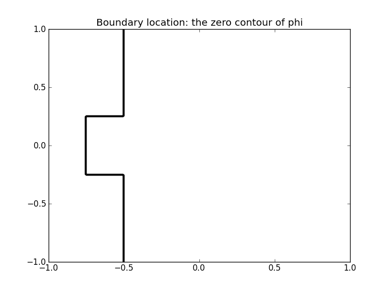
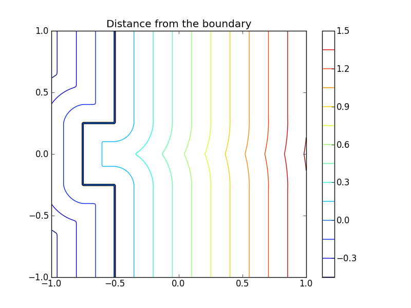
The boundary is specified as the zero contour of a scalar function phi:
>>> import numpy as np
>>> import pylab as pl
>>> X, Y = np.meshgrid(np.linspace(-1,1,200), np.linspace(-1,1,200))
>>> phi = -1 * np.ones_like(X)
>>> phi[X > -0.5] = 1
>>> phi[np.logical_and(np.abs(Y) < 0.25, X > -0.75)] = 1
>>> d = skfmm.distance(phi, dx=1e-2)
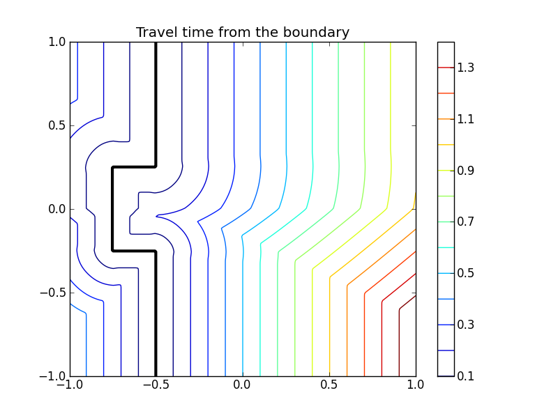
scikit-fmm can also calculate travel times from an interface
given an array containing the interface propogation speed at each
point. Using the same initial interface position as above we set the
interface propagation speed to be 1.5 times greater in the upper half
of the domain.
>>> speed = np.ones_like(X)
>>> speed[Y > 0] = 1.5
>>> t = skfmm.travel_time(phi, speed, dx=1e-2)
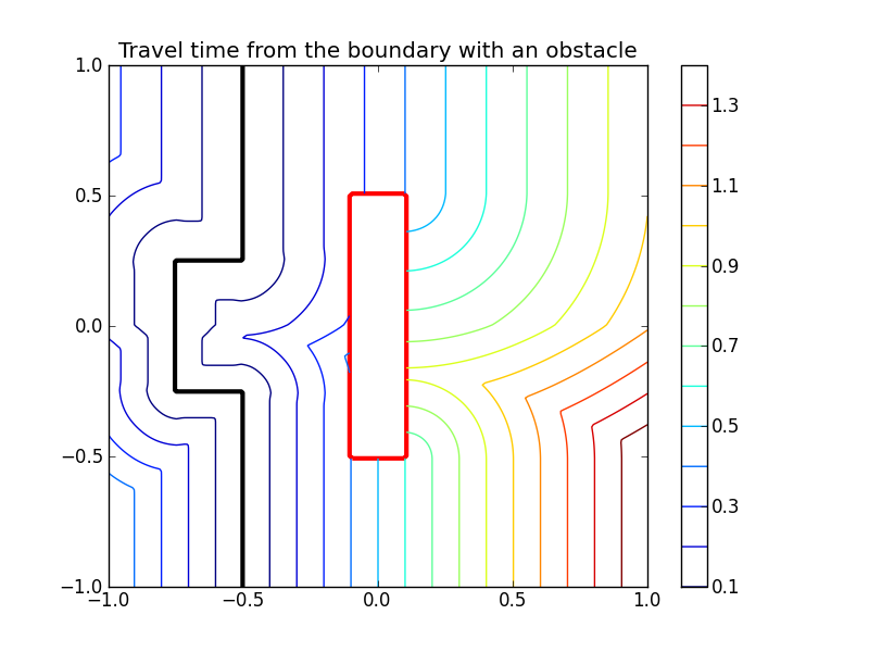
Consider an obstacle within which the speed is vanishing. In principle this may
lead to singularities (division by zero) in the update algorithm. Therefore,
both travel_time() and distance() support masked arrays for
input. This allows an obstacle to be introduced. (Note that if the speed in a cell
is less than machine precision, a cell is masked internally to prevent division by 0.)
>>> mask = np.logical_and(abs(X) < 0.1, abs(Y) < 0.5)
>>> phi  = np.ma.MaskedArray(phi, mask)
>>> t    = skfmm.travel_time(phi, speed, dx=1e-2)
The distance function, travel time or extension velocities can be limited to with in a narrow band around the zero contour by specifying the narrow keyword.
>>> phi = -1 * np.ones_like(X)
>>> phi[X > -0.5] = 1
>>> phi[np.logical_and(np.abs(Y) < 0.25, X > -0.75)] = 1
>>> d = skfmm.distance(phi, dx=1e-2, narrow=0.3)
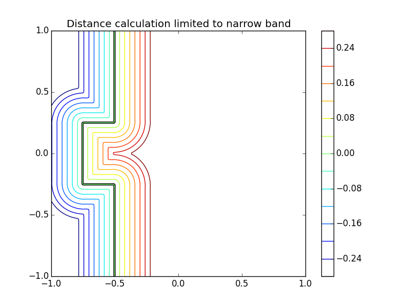
The full example is in examples/2d_example.py. Example Listing
An example of using periodic boundary conditions.
>>> X, Y = np.meshgrid(np.linspace(-1,1,501), np.linspace(-1,1,501))
>>> phi = (X+0.8)**2+(Y+0.8)**2 - 0.01
>>> speed = 1+X**2+Y**2
>>> skfmm.distance(phi, dx=2.0/500)
>>> skfmm.distance(phi, dx=2.0/500, periodic=True)
>>> skfmm.travel_time(phi, speed, dx=2.0/500, periodic=(1,0))
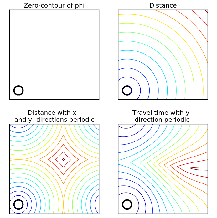
The full example is in examples/boundaryconditions_example.py Example Listing
An example of using scikit-fmm to compute extension velocities.
>>> N     = 150
>>> X, Y  = np.meshgrid(np.linspace(-1, 1, N), np.linspace(-1, 1, N))
>>> r     = 1.75
>>> dx    = 2.0 / (N - 1)
>>> phi   = (X) ** 2 + (Y+1.85) ** 2 - r ** 2
>>> speed = X + 1.25
>>> d, f_ext = extension_velocities(phi, speed, dx)
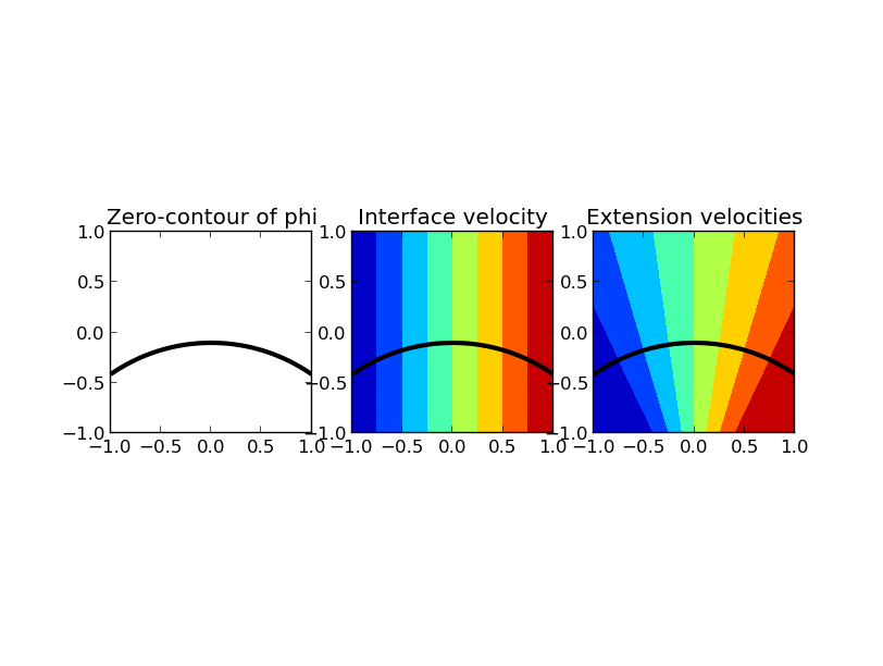
The full example is in examples/extension_velocities_example.py. Example Listing
Limitations:
scikit-fmm only works for regular Cartesian grids, but grid cells may
have a different (uniform) length in each dimension.
Function Reference
-
skfmm.distance(phi, dx=1.0, self_test=False, order=2, narrow=0.0, periodic=False)[source]¶ Return the signed distance from the zero contour of the array phi.
Parameters: phi : array-like
the zero contour of this array is the boundary location for the distance calculation. Phi can of 1,2,3 or higher dimension and can be a masked array.
dx : float or an array-like of len phi.ndim, optional
the cell length in each dimension.
self_test : bool, optional
if True consistency checks are made on the binary min heap during the calculation. This is used in testing and results in a slower calculation.
order : int, optional
order of computational stencil to use in updating points during the fast marching method. Must be 1 or 2, the default is 2.
narrow : float, optional
narrow band half-width. If this optional argument is specified the marching algorithm is limited to within a given narrow band. If far-field points remain when this condition is met a masked array is returned. The default value is 0.0 which means no narrow band limit.
periodic : bool or an array-like of len phi.ndim, optional
specifies whether and in which directions periodic boundary conditions are used. True sets periodic boundary conditions in all directions. An array-like (interpreted as True or False values) specifies the absence or presence of periodic boundaries in individual directions. The default value is False, i.e., no periodic boundaries in any direction.
Returns: d : an array the same shape as phi
contains the signed distance from the zero contour (zero level set) of phi to each point in the array. The sign is specified by the sign of phi at the given point.
-
skfmm.travel_time(phi, speed, dx=1.0, self_test=False, order=2, narrow=0.0, periodic=False)[source]¶ Return the travel from the zero contour of the array phi given the scalar velocity field speed.
Parameters: phi : array-like
the zero contour of this array is the boundary location for the travel time calculation. Phi can of 1,2,3 or higher dimension and can be a masked array.
speed : array-like, the same shape as phi
contains the speed of interface propagation at each point in the domain.
dx : float or an array-like of len phi.ndim, optional
the cell length in each dimension.
self_test : bool, optional
if True consistency checks are made on the binary min heap during the calculation. This is used in testing and results in a slower calculation.
order : int, optional
order of computational stencil to use in updating points during the fast marching method. Must be 1 or 2, the default is 2.
narrow : float, optional
narrow band half-width. If this optional argument is specified the marching algorithm is limited to travel times within a given value. If far-field points remain when this condition is met a masked array is returned. The default value is 0.0 which means no narrow band limit.
periodic : bool or an array-like of len phi.ndim, optional
specifies whether and in which directions periodic boundary conditions are used. True sets periodic boundary conditions in all directions. An array-like (interpreted as True or False values) specifies the absence or presence of periodic boundaries in individual directions. The default value is False, i.e., no periodic boundaries in any direction.
Returns: t : an array the same shape as phi
contains the travel time from the zero contour (zero level set) of phi to each point in the array given the scalar velocity field speed. If the input array speed has values less than or equal to zero the return value will be a masked array.
-
skfmm.extension_velocities(phi, speed, dx=1.0, self_test=False, order=2, ext_mask=None, narrow=0.0, periodic=False)[source]¶ Extend the velocities defined at the zero contour of phi, in the normal direction, to the rest of the domain. Extend the velocities such that grad f_ext dot grad d = 0 where where f_ext is the extension velocity and d is the signed distance function.
Parameters: phi : array-like
the zero contour of this array is the boundary location for the travel time calculation. Phi can of 1,2,3 or higher dimension and can be a masked array.
speed : array-like, the same shape as phi
contains the speed of interface propagation at each point in the domain.
dx : float or an array-like of len phi.ndim, optional
the cell length in each dimension.
self_test : bool, optional
if True consistency checks are made on the binary min heap during the calculation. This is used in testing and results in a slower calculation.
order : int, optional
order of computational stencil to use in updating points during the fast marching method. Must be 1 or 2, the default is 2.
ext_mask : array-like, the same shape as phi, optional
enables initial front values to be eliminated when calculating the value at the interface before the values are extended away from the interface.
narrow : float, optional
narrow band half-width. If this optional argument is specified the marching algorithm is limited to within a given narrow band. If far-field points remain when this condition is met a masked arrays are returned. The default value is 0.0 which means no narrow band limit.
periodic : bool or an array-like of len phi.ndim, optional
specifies whether and in which directions periodic boundary conditions are used. True sets periodic boundary conditions in all directions. An array-like (interpreted as True or False values) specifies the absence or presence of periodic boundaries in individual directions. The default value is False, i.e., no periodic boundaries in any direction.
Returns: (d, f_ext) : tuple
a tuple containing the signed distance function d and the extension velocities f_ext.
-
class
skfmm.heap(max_size, self_test=False)[source]¶ Note
Using this class is not required to use
distance(),travel_time()orextension_velocities(). It is provided for experimenting with fast marching algorithms.This class implements a binary min heap (or heap queue) to support the fast marching algorithm. A min heap is a list which has the property that the smallest element is always the first element. http://en.wikipedia.org/wiki/Binary_heap
This class differs from the heap queue (
heapq) in the Python standard library because it supports changing the value of elements in the heap and maintains forward and backward ids.The fast marching method uses this data structure to track elements in the solution narrow band. The fast marching method needs to know which element in the narrow band is nearest the zero level-set at each iteration. When a new point enters the solution narrow band the element is added to the heap.
New elements (an address and an initial value) are added to the heap with the
push()method. Thepush()method returns an integer (aheap_id) which is used to update the value of the element.As the solution evolves, the distance of points already in the heap are updated via the
update()method. Theupdate()method takes theheap_idreturned by thepush()along with a new distance value.The smallest element is taken off the heap with the
pop()method. The address and value of the top element is returned.The constructor for heap needs to know the number of elements that will enter the heap.
>>> from skfmm import heap
>>> h = heap(10)
>>> h.push(10,0.2)
0
>>> h.push(11,0.3)
1
>>> h.push(12,0.1)
2
>>> h.peek()
0.1
>>> h.update(1, 0.01)
>>> h.peek()
0.01
>>> h.pop()
(11, 0.01)
>>> h.pop()
(12, 0.1)
>>> h.pop()
(10, 0.2)
>>> assert h.empty()
Methods
-
peek()[source]¶ Returns the top (smallest) value on the heap without removing it.
Returns: value : float
The top (smallest) value on the heap.
-
pop()[source]¶ Remove and return the address and value of the top element on the heap.
Returns: (addr, value) : tuple
A tuple of the address given when the element was pushed onto the heap and the current value of the element.
-
push(addr, value)[source]¶ Add a value to the heap, give an address and a value.
Parameters: addr : int
An id number which is returned when the element is popped off the heap.
value : float
An initial numerical value for this element.
Returns: heap_id : int
An id number into the heap used to update the value of this element. The value of a point in the heap can be updated by calling
update()with this id and a new value.
-