1. System

Note

It is assumed that pyofss has been imported using

>>> from pyofss import *

Every pyofss simulation begins with a system. To generate a system with a default domain:

>>> sys = System()

which is equivalent to

>>> sys = System( Domain() )

Various modules may be added to the system such as pulse generators, fibres, and filters. Once a module has been generated, add it to the system. As an example, to construct a Gaussian pulse generator and add it to the system:

>>> gaussian = Gaussian()
>>> sys.add( gaussian )

It is also possible to directly add a module using:

>>> sys.add( Gaussian() )

Once all modules have been added, run the simulation

>>> sys.run()

This generates a field which is modified by each module it propagates through.

The output field may be accessed using:

>>> sys.field

A field will generally be an array of complex values. There are utility functions which allow calculating the temporal and spectral power:

>>> P_t = temporal_power( sys.field )
>>> P_nu = spectral_power( sys.field )

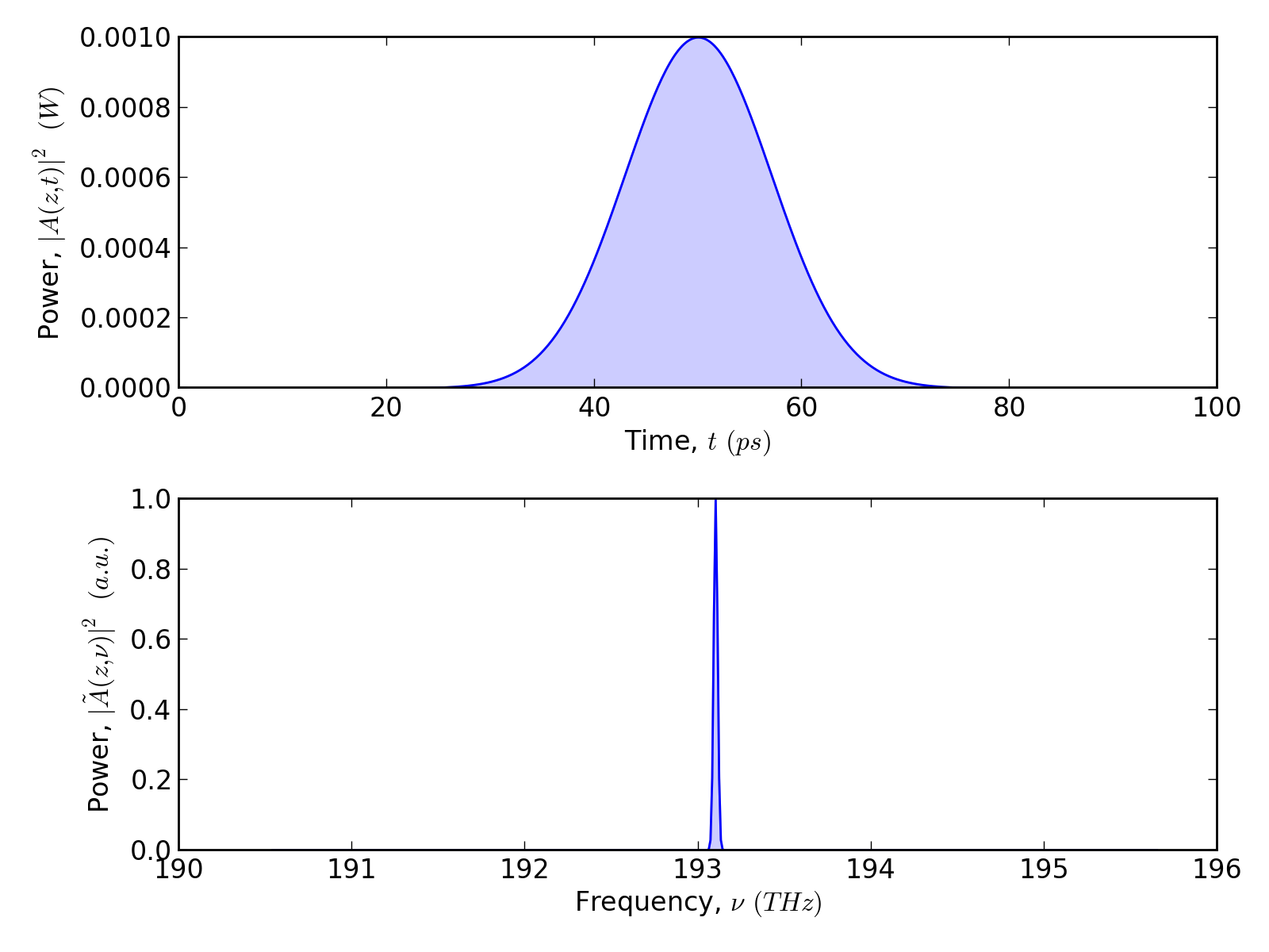
There is also a plotter which allows a range of plots to be generated. As an example, the temporal and spectral power of the resulting field may be plotted in a “double” plot:

from pyofss import *
sys = System( Domain() )
sys.add( Gaussian() )
sys.run()
double_plot( sys.domain.t, temporal_power(sys.field),
             sys.domain.nu, spectral_power(sys.field, True),
             labels['t'], labels['P_t'], labels['nu'], labels['P_nu'] )

(Source code, png, hires.png, pdf)