1. Quick Start

pymeigo does not expose all of the MEIGOR functions. Right now it exposes the VNS and ESS algorithms (not the parallel version). The two searcj algorithms can be found in essR() and rvnsd_hamming().

In addition, pymeigo provides 2 example of functions to play with that can be found in funcs module. One of them is called rosen() and we will use it in this quickstart. First, just import everything from the package pymeigo:

from pymeigo import *

You can optimise either Python or R functions. In order to optimise a R function, it must be available from the Python interface. Although it is possible to optimise a R function, the idea of pymeigo is to be able to optimise python functions using MEIGOR. Therefore, this tutorial focues only on how to optimise python functions.

To optimise a python function, one must convert the python function into a R object. We provide a function to perform this task easily via the pymeigo.funcs.pyfunc2R() function. For instance, consider the following python function:

def rosen(x):
    """Rosenbrock Banana function as a cost function
     (as in the R man page for optim())
    """
    x1 = x[0]
    x2 = x[1]
    return 100 * (x2 - x1 * x1)**2 + (1 - x1)**2

If you pass it directly to R, you will get an error. You must convert it into a R object as follows:

# wrap the function rosen so it can be exposed to R
rosen_for_r = pyfunc2R(rosen)

Then, you can optimisize the rosen_for_r() function as follows:

res = essR(f=rosen_for_r, x_U=[2,2], x_L=[-1,-1])

where x_U and x_L are the upper and lower bounds of the 2 parameters used by the rosen functio. The output of the algorithm being:

------------------------------------------------------------------------------
 essR - Enhanced Scatter Search in R
<c> IIM-CSIC, Vigo, Spain -  email: gingproc@iim.csic.es
------------------------------------------------------------------------------

Refset size automatically calculated: 6
Number of diverse solutions automatically calculated: 20
Initial Pop: NFunEvals: 25 Bestf: 2.322351 CPUTime: 0.005 Mean: 51.29905
Iteration: 1 NFunEvals: 62 Bestf: 0.05619965 CPUTime: 0.011 Mean: 1.659653
Iteration: 2 NFunEvals: 98 Bestf: 0.03821879 CPUTime: 0.017 Mean: 1.189044
...
Iteration: 28 NFunEvals: 998 Bestf: 3.634548e-05 CPUTime: 0.153 Mean: 0.000100323
Iteration: 29 NFunEvals: 1033 Bestf: 2.398931e-05 CPUTime: 0.157 Mean:  8.80343e-05

Maximum number of function evaluations achieved
Best solution value 2.398931e-05
Decision vector 1.000646 1.001778
CPU time 0.158
Number of function evaluations 1033

you can then introspect the results as you would do in R by looking at the returned R object:

>>> res.names
Out[21]:
<StrVector - Python:0x7217cf8 / R:0x67ea5b8>
['f', 'x', 'time', ..., 'end_..., 'cpu_..., 'Refs...]

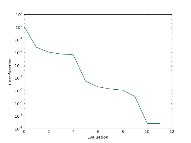
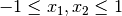
For instance, f contains the cost function results:

from pymeigo import *
res = essR(f=rosen_for_r, x_U=[2,2], x_L=[-1,-1])

from pylab import plot, xlabel, ylabel, semilogy
plot(res.f)
xlabel("Evaluation")
ylabel("Cost function")
semilogy(res.f)

(Source code, png, hires.png, pdf)

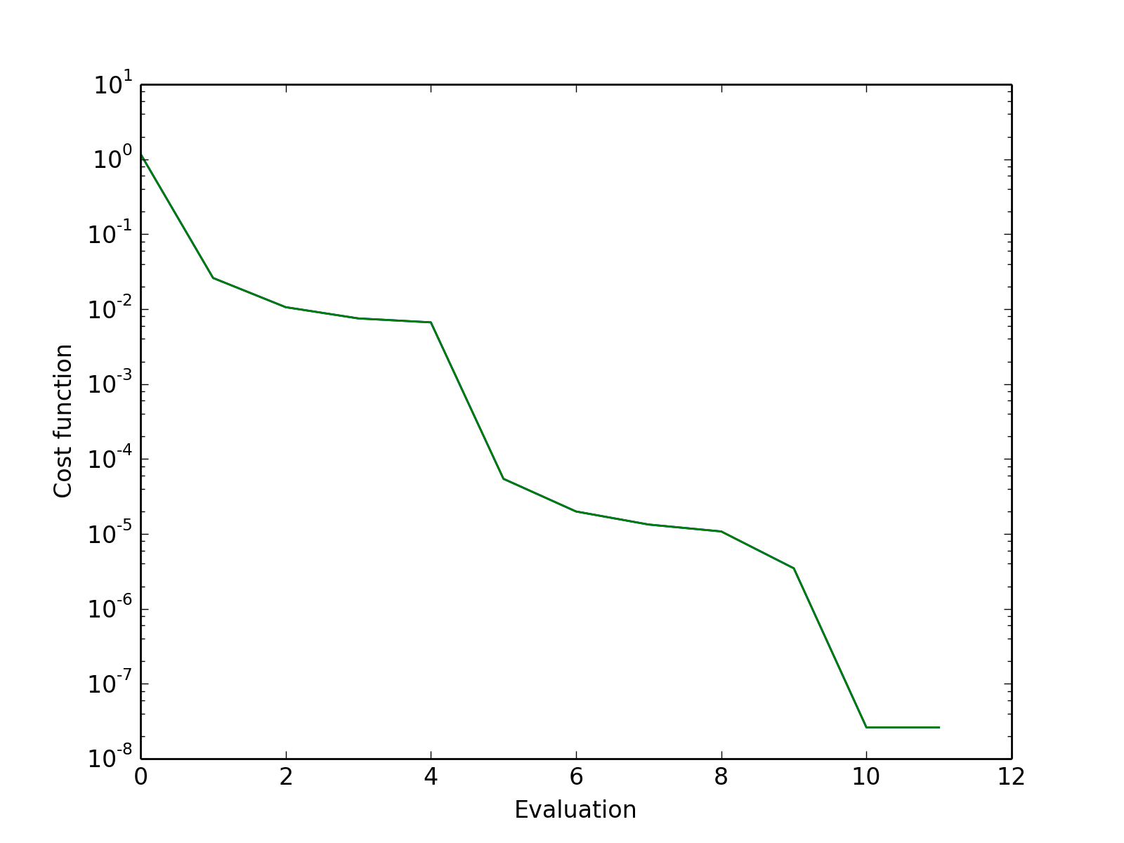
Finally, there is a simple class prototype equivalent to the code above that is provided:

from pymeigo import ESS, rosen_for_r
m = ESS(f=rosen_for_r)
m.run(x_U=[2,2], x_L=[-1,-1])
m.plot()

(Source code, png, hires.png, pdf)

2. Example

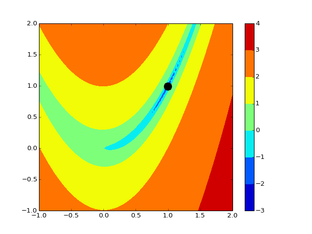
2.1. Rosen function

In the following example, we consider the rosen function (see figure below), which has a minimum at x=1, y=1. First, we search for the best solution. Second, we plot the function. Third, we plot the best solution found in step 1 (black circle).

# 1. optimisation
from pylab import *
from pymeigo import *
m = ESS(f=rosen_for_r)
m.run(x_U=[2,2], x_L=[-1,-1])

# plot rosen function
x = linspace(-1,2,100)
y = linspace(-1,2,100)
X,Y = meshgrid(x,y)
Z = rosen([X,Y])
contourf(X, Y, log10(Z))
colorbar()

# plot the best solution found
plot(m.res.xbest[0], m.res.xbest[1], 'ok', markersize=15)

(Source code, png, hires.png, pdf)

You can also use the VNS algorithm:

>>> from pymeigo import *
>>> m = VNS(f=rosen_for_r)
>>> m.run(x_U=[2,2], x_L=[-1,-1])
>>> m.res.xbest
[1,1]

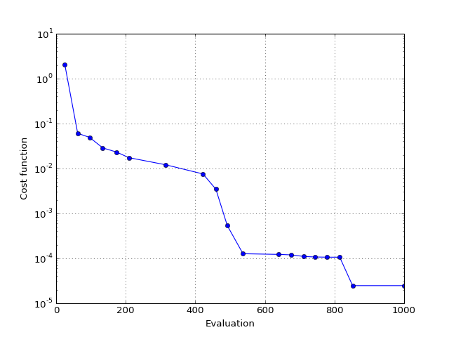
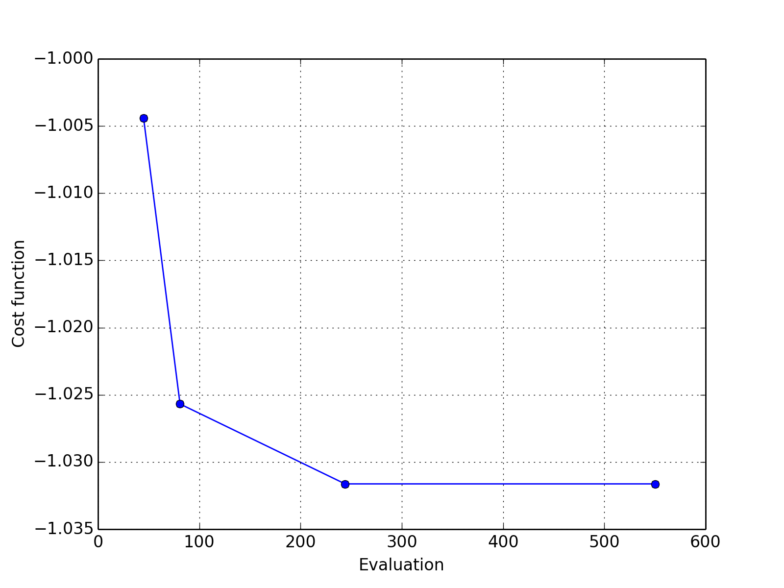
2.2. Unconstrained function

In pymeigo, we provide some examples to play with (mod:pymeigo.funcs). The first one is a unconstrained problem defined as follows:

subject to:

The objective function is provided in pymeigo (example_unconstrained) and constraints are provided when running the optimisation. Note that this problem has 2 solutions and the following example returns only one solution. In this example, we also use the maxeval and ndiverse parameters as well as a local solver called DHC (See the R documentation of MEIGOR). You can also simply use the default parameters.

>>> from pymeigo import *
>>> m = ESS(f=example_unconstrained_for_r)
>>> m.run(x_U=[1, 1], x_L=[-1, -1], maxeval=500, ndiverse=40,local_solver="DHC")
>>> m.plot()
>>> list(m.res.xbest)
[0.08984201089521965, -0.7126564013657124]

(Source code, png, hires.png, pdf)