
The Leaf Graph Language
LGL is a formal language whose aim is to define graphs by writing a code that is as readable as possible. It supports two main coding style: one being very easy to write but less readable, the other one being a bit more complex to write but resulting into an almost visual representation of a graph. In the following paragraphs the two styles are described by means of examples. lglc is the LGL compiler, whose output is a graph in Dot language. lglc is internally used by pyleaf.Designing an LGL graph the easy way
You can define an LGL graph by composition of node chains, the latter being very straightforward to code. A simple chain is defined this way:
1 -> 2 -> 3;
representing the following graph:
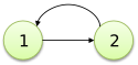
You can add a branch to the previous graph rooted in node 2 using the following syntax:
@2 -> 4;
The latter code, together with the former, generates the following
graph: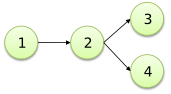
By composing graphs this way any graph can be designed very easily.
LGL syntax by examples
The following is a table showing more advanced statements to define graphs in LGL. It can be used to make LGL code both more readable and powerful (few instructions to build complex graph structures).| Operation | LGL code | Result | Chain |
1 -> 2 -> 3;
|
|
|
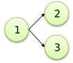
Fork 2 is said "left child", 3 is said "right child" |
  /2
1<
  \3
;
|
|
|
Fork to fork with void node |
     /4
   2<
  /  \5
1<
  \  /6
   .<
     \7
;
|
|
| Node set |
1, 2, 3; |

|
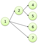
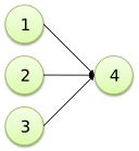
| Set to node |
1, 2, 3 -> 4; |
|
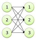
| Set to set |
1, 2, 3 -> 4, 5, 6; |

|
| Node reference |
1 -> 2 -> @1; |
|
| Named object: |
G: 1, 2, 3; |
|
| Object copy |
G: 1, 2, 3; G -> G; |
|
| Object reference |
G: 1, 2, 3; G -> @G; |
|
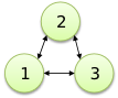
Forking forks
There are simple ways to edit any kind of graph with LGL. In some situations, however, editing an existing LGL graph retaining graph readability may require some practice. Consider the following graph:/B A < \C ;
   /B
A <
   \  /D
    C<
      \E
;
   /B
A <
   \      /F
        D<
       /  \G
     C<
       \E
;
There are at least three ways to avoid the gap. One is to rotate the sub-tree rooted in C (switch left child with right child), but this can be complicated if the graph is big. A simpler solution is the following:
   /B
A <
   \   /D -> F, G
     C<
       \E
;
Finally, note that in order to expand the other branch one needs to do as follows:
      /E
    B<
   /  \  /F
       D<
         \G

A <
   \C
;
Improving readability
Suppose to have the following LGL graph:
                                            / MDS_2D -> visualize2D
load_data -> preprocess_data -> pca_reduce <
                                            \      / hierarchical_clustering
                                                 .<
                                                /  \ kmeans_clustering
                                             . <
                                                \ MDS_3D -> visualize3D
;
- It tends to grow too much horizontally (consider what happens on large protocols).
- It has a disjoint branch (there is no visual clue connecting the node pca_reduce to its right subtree).
Exploiting newlines, the protocol can be rewritten this way:
                      / MDS_2D
                         -> visualize2D
load_data
   -> preprocess_data
      -> pca_reduce <
                     \      / hierarchical_clustering
                          .<
                         /  \ kmeans_clustering
                      . <
                         \ MDS_3D
                            -> visualize3D
;
                       / MDS_2D
                      |   -> visualize2D
load_data             |
   -> preprocess_data |
      -> pca_reduce  <
                      \     / hierarchical_clustering
                       |  .<
                       | /  \ kmeans_clustering
                       .<
                         \ MDS_3D
                            -> visualize3D
;
Node flags and attributes
Special flags can be associated with nodes enclosing them into "[]" brackets, as in the following example:download_data[F] -> analyze -> save_results [F];
LGL also supports node attributes through attribute = value pairs. They can be also mixed with flags, like in the following example:
download_data[F, color=green] -> analyze -> save_results [F];