Indices and tables
Overview


pygslodeiv2 provides a Python binding to the Ordinary Differential Equation integration routines exposed by the odeiv2 interface of GSL - GNU Scientific Library. The odeiv2 interface allows a user to numerically integrate (systems of) differential equations.
The following stepping functions are available:
- rk2
- rk4
- rkf45
- rkck
- rk8pd
- rk1imp
- rk2imp
- rk4imp
- bsimp
- msadams
- msbdf
Note that all implicit steppers (those ending with “imp”) and msbdf require a user supplied callback for calculating the jacobian.
Documentation
Autogenerated API documentation for latest stable release is found here: https://pythonhosted.org/pygslodeiv2 (and development docs for the current master branch are found here: http://hera.physchem.kth.se/~pygslodeiv2/branches/master/html).
Installation
Simplest way to install is to use the conda package manager:
$ conda install -c bjodah pygslodeiv2 pytest
$ python -m pytest --pyargs pygslodeiv2
tests should pass.
Binary distribution is available here: https://anaconda.org/bjodah/pygslodeiv2, conda recipes for stable releases are available here: http://hera.physchem.kth.se/~pygslodeiv2/conda-recipes.
Source distribution is available here (requires GSL v1.16 or v2.1 shared lib with headers): https://pypi.python.org/pypi/pygslodeiv2 (with mirrored files kept here: http://hera.physchem.kth.se/~pygslodeiv2/releases)
Examples
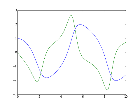
The classic van der Pol oscillator (see examples/van_der_pol.py)
>>> import numpy as np
>>> from pygslodeiv2 import integrate_predefined  # also: integrate_adaptive
>>> mu = 1.0
>>> def f(t, y, dydt):
...     dydt[0] = y[1]
...     dydt[1] = -y[0] + mu*y[1]*(1 - y[0]**2)
...
>>> def j(t, y, Jmat, dfdt):
...     Jmat[0, 0] = 0
...     Jmat[0, 1] = 1
...     Jmat[1, 0] = -1 -mu*2*y[1]*y[0]
...     Jmat[1, 1] = mu*(1 - y[0]**2)
...     dfdt[0] = 0
...     dfdt[1] = 0
...
>>> y0 = [1, 0]; dt0=1e-8; t0=0.0; atol=1e-8; rtol=1e-8
>>> tout = np.linspace(0, 10.0, 200)
>>> yout, info = integrate_predefined(f, j, y0, tout, dt0, atol, rtol,
...                                   method='bsimp')  # Implicit Bulirsch-Stoer
>>> import matplotlib.pyplot as plt
>>> series = plt.plot(tout, yout)
>>> plt.show()
For more examples see examples/, and rendered jupyter notebooks here: http://hera.physchem.kth.se/~pygslodeiv2/branches/master/examples
License
The source code is Open Source and is released under GNU GPL v3. See LICENSE for further details. Contributors are welcome to suggest improvements at https://github.com/bjodah/pygslodeiv2