Randomized Designs

In this section, the following kinds of randomized designs will be described:

• Latin-Hypercube

Hint

All available designs can be accessed after a simple import statement:

>>> from pyDOE import *

Latin-Hypercube (lhs)

Latin-hypercube designs can be created using the following simple syntax:

>>> lhs(n, [samples, criterion, iterations])

where

• n: an integer that designates the number of factors (required)
• samples: an integer that designates the number of sample points to generate for each factor (default: n)
• criterion: a string that tells lhs how to sample the points (default: None, which simply randomizes the points within the intervals):
  • “center” or “c”: center the points within the sampling intervals
  • “maximin” or “m”: maximize the minimum distance between points, but place the point in a randomized location within its interval
  • “centermaximin” or “cm”: same as “maximin”, but centered within the intervals
  • “correlation” or “corr”: minimize the maximum correlation coefficient

The output design scales all the variable ranges from zero to one which can then be transformed as the user wishes (like to a specific statistical distribution using the scipy.stats.distributions ppf (inverse cumulative distribution) function. An example of this is shown below.

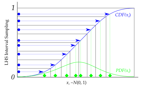
For example, if I wanted to transform the uniform distribution of 8 samples to a normal distribution (mean=0, standard deviation=1), I would do something like:

>>> from scipy.stats.distributions import norm
>>> lhd = lhs(2, samples=5)
>>> lhd = norm(loc=0, scale=1).ppf(lhd)  # this applies to both factors here

Graphically, each transformation would look like the following, going from the blue sampled points (from using lhs) to the green sampled points that are normally distributed:

Examples

A basic 4-factor latin-hypercube design:

>>> lhs(4, criterion='center')
array([[ 0.875,  0.625,  0.875,  0.125],
       [ 0.375,  0.125,  0.375,  0.375],
       [ 0.625,  0.375,  0.125,  0.625],
       [ 0.125,  0.875,  0.625,  0.875]])

Let’s say we want more samples, like 10:

>>> lhs(4, samples=10, criterion='center')
array([[ 0.05,  0.05,  0.15,  0.15],
       [ 0.55,  0.85,  0.95,  0.75],
       [ 0.25,  0.25,  0.45,  0.25],
       [ 0.45,  0.35,  0.75,  0.45],
       [ 0.75,  0.55,  0.25,  0.55],
       [ 0.95,  0.45,  0.35,  0.05],
       [ 0.35,  0.95,  0.05,  0.65],
       [ 0.15,  0.65,  0.55,  0.35],
       [ 0.85,  0.75,  0.85,  0.85],
       [ 0.65,  0.15,  0.65,  0.95]])

Customizing with Statistical Distributions

Now, let’s say we want to transform these designs to be normally distributed with means = [1, 2, 3, 4] and standard deviations = [0.1, 0.5, 1, 0.25]:

>>> design = lhs(4, samples=10)
>>> from scipy.stats.distributions import norm
>>> means = [1, 2, 3, 4]
>>> stdvs = [0.1, 0.5, 1, 0.25]
>>> for i in xrange(4):
...     design[:, i] = norm(loc=means[i], scale=stdvs[i]).ppf(design[:, i])
...
>>> design
array([[ 0.84947986,  2.16716215,  2.81669487,  3.96369414],
       [ 1.15820413,  1.62692745,  2.28145071,  4.25062028],
       [ 0.99159933,  2.6444164 ,  2.14908071,  3.45706066],
       [ 1.02627463,  1.8568382 ,  3.8172492 ,  4.16756309],
       [ 1.07459909,  2.30561153,  4.09567327,  4.3881782 ],
       [ 0.896079  ,  2.0233295 ,  1.54235909,  3.81888286],
       [ 1.00415   ,  2.4246118 ,  3.3500082 ,  4.07788558],
       [ 0.91999246,  1.50179698,  2.70669743,  3.7826346 ],
       [ 0.97030478,  1.99322045,  3.178122  ,  4.04955409],
       [ 1.12124679,  1.22454846,  4.52414072,  3.8707982 ]])

Note

Methods for “space-filling” designs and “orthogonal” designs are in the works, so stay tuned! However, simply increasing the samples reduces the need for these anyway.

More Information

If the user needs more information about appropriate designs, please consult the following articles on Wikipedia:

• Latin-Hypercube designs

There is also a wealth of information on the NIST website about the various design matrices that can be created as well as detailed information about designing/setting-up/running experiments in general.

Any questions, comments, bug-fixes, etc. can be forwarded to the author.