Effect of initialization on accuracy of fit

An optimization procedure is used when computing the diffusion matrix from diffusion profiles. The function to be minimized has typically several local minima, since it is a complicated (non-quadratic and non-convex) function of a large number of parameters. The algorithm looks for a local minimum, using a gradient descent from the initial guess of the diffusion matrix. Therefore, it is possible that the algorithm returns a diffusion matrix very different from the one that is looked for, if the initial guess is very far from the ground truth.

For more information about non-linear least-squares optimization, please see https://en.wikipedia.org/wiki/Non-linear_least_squares

In this example, we show that a random initial condition, with a correct order of magnitude of the largest eigenvalue, results in a correct estimation in most cases. Only when the orientation of the dominant eigenvector is very far (almost perpendicular) to the true orientation, a different local minimum is sometimes found, resulting in a bad fit and a wrong estimation of the diffusion matrix.

import numpy as np
import matplotlib.pyplot as plt
from multidiff import compute_diffusion_matrix, create_diffusion_profiles

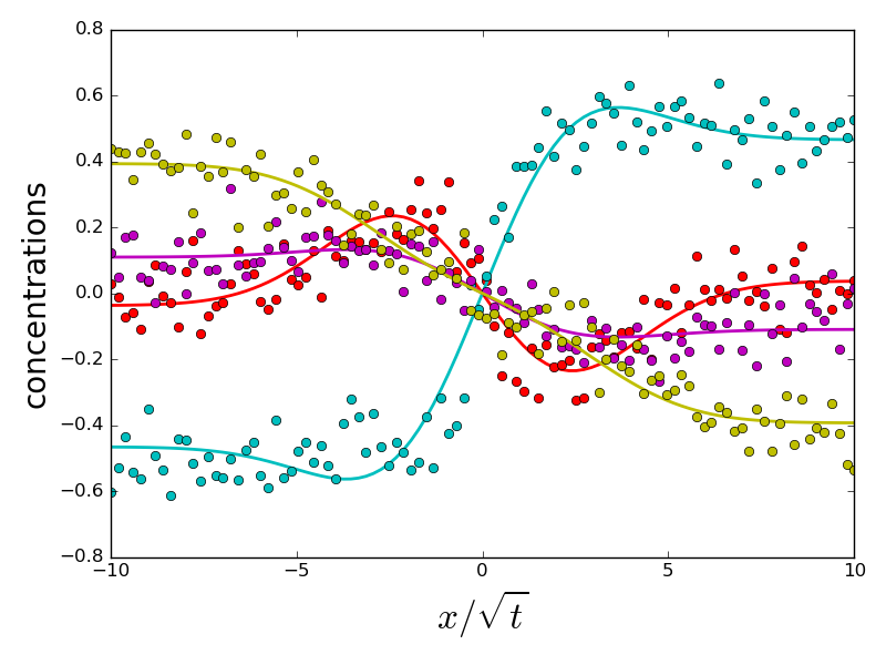
A system with 4 components is used here. The diffusion matrix is quite

ill-conditioned, since the ratio between largest and smallest eigenvalues is 40. The dominant eigenvector corresponds to the exchange of the two last components. Five different exchange experiments are generated (in theory, 3 experiments would be enough, but the optimization is better constrained

 with more data).

n_comp = 4 # number of components
# Ground truth diffusion matrix
diags = np.array([0.5, 5., 20])
P = np.matrix([[ 1,  1,  0],
               [-1,  0,  0],
               [ 0, -1, -1]])
# Measurement points
xpoints_exp1 = np.linspace(-10, 10, 100)
x_points = [xpoints_exp1] * 5


# Which components are exchanged in each experiment
exchange_vectors = np.array([[ 0,  1,  1,  1,  0],
                             [ 1, -1,  0,  0,  1],
                             [-1,  0, -1,  0,  0],
                             [ 0,  0,  0, -1, -1]])
noise = 0.07

concentration_profiles = create_diffusion_profiles((diags, P), x_points,
        exchange_vectors, noise_level=noise)

In order to investigate the robustness of the solution with respect to the initial value of the diffusion matrix, we generate random values for eigenvalues and eigenvectors. The order of magnitude of eigenvalues is chosen to be comparable to the largest eigenvalue. Note that the largest eigenvalue can be easily estimated from experimental data, using the largest diffusion distance observed in all experiments.

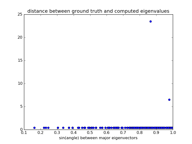
In order to estimate the proximity between the initialization and the diffusion matrix, we compute the angle between the leading eigenvector of the initialization, and of the diffusion matrix.

np.random.seed(0)
nb_iter = 200
errors = np.empty((nb_iter, n_comp - 1))

diags_all = np.empty((nb_iter, n_comp - 1))
eigvecs_all = np.empty((nb_iter, n_comp - 1, n_comp - 1))
distances = np.empty(nb_iter)

do_plot = True


def angle_between(v1, v2):
    """ Returns the angle in radians between vectors 'v1' and 'v2'::

            >>> angle_between((1, 0, 0), (0, 1, 0))
            1.5707963267948966
            >>> angle_between((1, 0, 0), (1, 0, 0))
            0.0
            >>> angle_between((1, 0, 0), (-1, 0, 0))
            3.141592653589793
    """
    v1_u = v1 / np.linalg.norm(v1) # unit vector
    v2_u = v2 / np.linalg.norm(v2)
    return np.arccos(np.clip(np.dot(v1_u, v2_u), -1.0, 1.0))


for i in range(nb_iter):
    diags_init = 20 * np.random.random(3)
    P_init = np.random.random(9).reshape((3, 3)) - 0.5
    diags_res, eigvecs, _, _, _ = (
            compute_diffusion_matrix((diags_init, P_init), x_points,
                                        concentration_profiles, plot=False))
    errors[i] = np.abs(np.sort(diags_res) - diags) / diags
    diags_all[i] = diags_init
    eigvecs_all[i] = P_init
    indices = np.argsort(diags_init)
    eigs_sorted = P_init[:, indices]
    distances[i] = [np.sin(angle_between(eig1, eig2)) for (eig1, eig2) in
                            zip(eigs_sorted.T, np.array(P).T)][-1]
    if errors[i].sum() > 1 and do_plot:
        _ = compute_diffusion_matrix((diags_init, P_init), x_points,
                                        concentration_profiles, plot=True)
        do_plot = False

• 
• 
• 
• 
• 

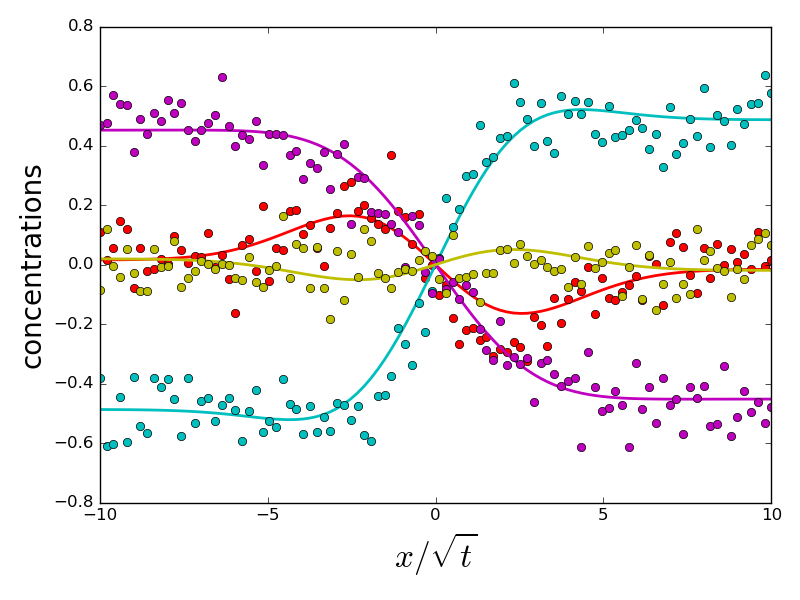
A very large majority of initializations converge to the same result, for

which the error on eigenvalues is small and due to experimental noise. However, a handful of initializations converge to a different energy minimum, for which eigenvalues and eigenvectors are very different from the ground truth. All problematic eigenvalues have a dominant eigenvector which is almost perpendicular to the eigenvector of the ground truth. Therefore, choosing an initialization with a correct orientation of the dominant eigenvector is important for a correct fit.

However, since most initializations result in a correct solution, an

 efficient strategy can be to use several inttializations chosen at random,

and to check whether the same solution is found consistently.

plt.figure()
plt.plot(distances, errors.sum(axis=1), 'o')
plt.xlabel('sin(angle) between major eigenvectors')
plt.title('distance between ground truth and computed eigenvalues')


plt.show()

Total running time of the script: ( 2 minutes 46.139 seconds)