Fitting multidiffusion profiles for three components

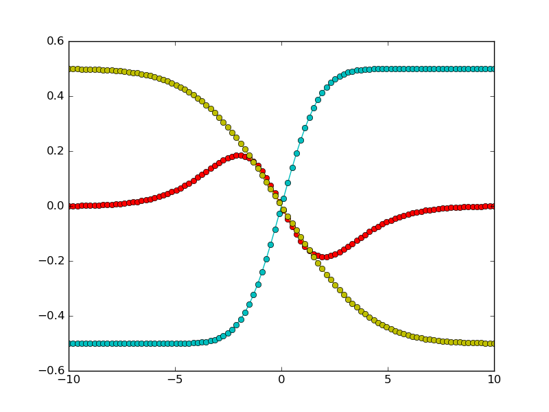
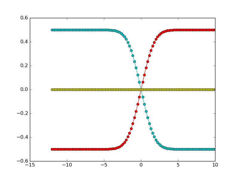
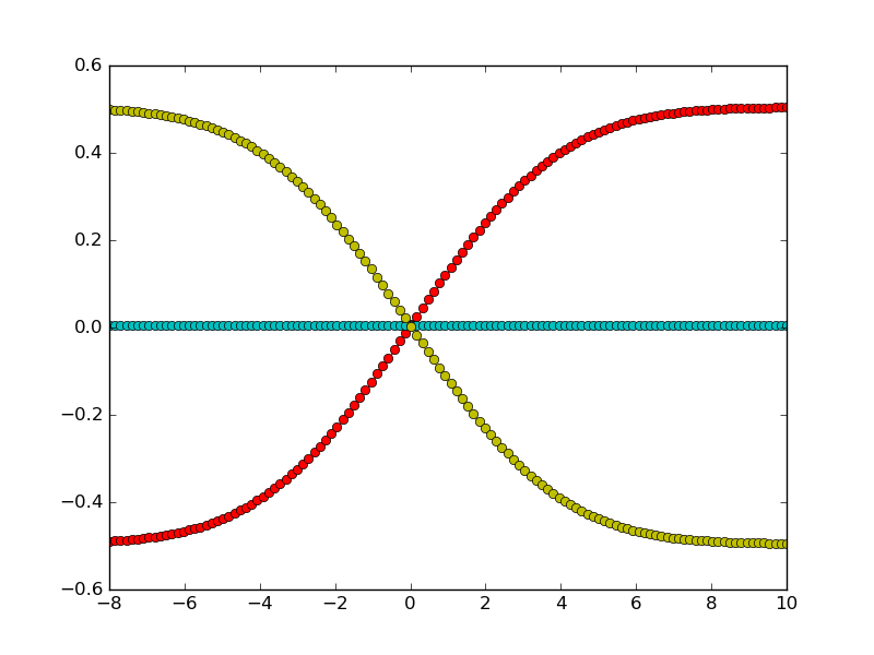
A typical fitting procedure is shown in this example. Synthetic diffusion profiles are generated for a system with three components, and three different different exchange experiments. Uphill diffusion is observed for one of the exchange experiments. For a moderate noise, we see that the fitting procedure results in an accurate estimate of the diffusion matrix.

import numpy as np
import matplotlib.pyplot as plt
from multidiff import compute_diffusion_matrix, create_diffusion_profiles

First we generate synthetic data, with three components. The diffusion matrix has two eigenvalues with quite different magnitudes. Exchange vectors correspond to the exchange of the three possible pairs of components (meaning that each endmember is enriched in one component and poorer in another, compared to the other endmember).

n_comps = 2

diags = np.array([1, 5])
P = np.matrix([[1, 1], [-1, 0]])

It is possible to have different measurement points for the different experiments. Also note that measurement points don’t have to be symmetric around 0.

xpoints_exp1 = np.linspace(-10, 10, 100)
xpoints_exp2 = np.linspace(-12, 10, 100)
xpoints_exp3 = np.linspace(-8, 10, 120)
x_points = [xpoints_exp1, xpoints_exp2, xpoints_exp3]

Let us now define the exchange vectors. Each column corresponds to an experiment: e.g. the first column represents the exchange of the first two components.

exchange_vectors = np.array([[0, 1, 1],
               [1, -1, 0],
               [-1, 0, -1]])


concentration_profiles = create_diffusion_profiles((diags, P), x_points,
                                                    exchange_vectors,
                                                    noise_level=0.0)

The algorithm needs an initial guess for the diffusion matrix. Here we give an initialization that is quite far from the looked-for diffusion matrix. Nevertheless, the result of the fit is quite good.

diags_init = np.array([1, 1])
P_init = np.eye(2)
diags_res, eigvecs, _, _, _ = compute_diffusion_matrix((diags_init, P_init),
                               x_points,
                               concentration_profiles, plot=True)

print("True eigenvalues: ", diags)

print("Fitted eigenvalues: ", diags_res)

print("True eigenvectors: ", P)

print("Fitted eigenvalues: ", eigvecs)

plt.show()

• 
• 
• 

Out:

True eigenvalues:  [1 5]
Fitted eigenvalues:  [ 5.  1.]
True eigenvectors:  [[ 1  1]
 [-1  0]]
Fitted eigenvalues:  [[  9.99999999e-01   9.99999999e-01]
 [  6.33327769e-10  -1.00000000e+00]
 [ -1.00000000e+00   9.02231595e-10]]

Total running time of the script: ( 0 minutes 0.507 seconds)