What are Gaussian processes?
Often we have an inference problem involving \(n\) data,
where the \(\boldsymbol{x_i}\) are the inputs and the \(y_i\) are the targets. We wish to make predictions, \(y_*\), for new inputs \(\boldsymbol{x_*}\). Taking a Bayesian perspective we might build a model that defines a distribution over all possible functions, \(f: \mathcal{X} \rightarrow \mathbb{R}\). We can encode our initial beliefs about our particular problem as a prior over these functions. Given the data, \(\mathcal{D}\), and applying Bayes’ rule we can infer a posterior distribution. In particular, for any given \(\boldsymbol{x_*}\) we can calculate or approximate a predictive distribution over \(y_*\) under this posterior.
Gaussian processes (GPs) are probability distributions over functions for which this inference task is tractable. They can be seen as a generalisation of the Gaussian probability distribution to the space of functions. That is a multivariate Gaussian distribution defines a distribution over a finite set of random variables, a Gaussian process defines a distribution over an infinite set of random variables (for example the real numbers). GP domains are not restricted to the real numbers, any space with a dot product is suitable. Analagously to a multivariate Gaussian distribution, a GP is defined by its mean, \(\mu\), and covariance, \(k\). However for a GP these are themselves functions, \(\mu: \mathcal{X} \rightarrow \mathbb{R}\) and \(k: \mathcal{X} \times \mathcal{X} \rightarrow \mathbb{R}\). In all that follows we assume \(\mu(\boldsymbol{x}) = 0\) as without loss of generality as we can always shift the data to accommodate any given mean.
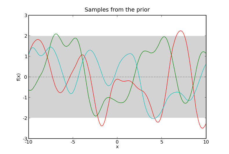
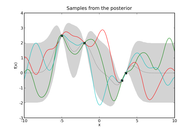
Samples from two Gaussian processes with the same mean and covariance functions. Here \(\mathcal{X} = \mathbb{R}\). The prior samples are taken from a Gaussian process without any data and the posterior samples are taken from a Gaussian process where the data are shown as black squares. The black dotted line represents the mean of the process and the gray shaded area covers twice the standard deviation at each input, \(x\). The coloured lines are samples from the process, or more accurately, samples at a finite number of inputs, \(x\), joined by lines.
The code to generate the above figures:
from numpy.random import seed
from infpy.gp import GaussianProcess, gp_1D_X_range, gp_plot_samples_from
from pylab import plot, savefig, title, close, figure, xlabel, ylabel

# seed RNG to make reproducible and close all existing plot windows
seed(2)
close('all')

#
# Kernel
#
from infpy.gp import SquaredExponentialKernel as SE
kernel = SE([1])

#
# Part of X-space we will plot samples from
#
support = gp_1D_X_range(-10.0, 10.01, .125)

#
# Plot samples from prior
#
figure()
gp = GaussianProcess([], [], kernel)
gp_plot_samples_from(gp, support, num_samples=3)
xlabel('x')
ylabel('f(x)')
title('Samples from the prior')
savefig('samples_from_prior.png')
savefig('samples_from_prior.eps')

#
# Data
#
X = [[-5.], [-2.], [3.], [3.5]]
Y = [2.5, 2, -.5, 0.]

#
# Plot samples from posterior
#
figure()
plot([x[0] for x in X], Y, 'ks')
gp = GaussianProcess(X, Y, kernel)
gp_plot_samples_from(gp, support, num_samples=3)
xlabel('x')
ylabel('f(x)')
title('Samples from the posterior')
savefig('samples_from_posterior.png')
savefig('samples_from_posterior.eps')
The covariance function, \(k\)
Assuming the mean function, \(\mu\), is 0 everywhere then our GP is defined by two quantities: the data, \(\mathcal{D}\); and its covariance function (sometimes referred to as its kernel), \(k\). The data is fixed so our modelling problem is exactly that of choosing a suitable covariance function. Given different problems we certainly wish to specify different priors over possible functions. Fortunately we have available a large library of possible covariance functions each of which represents a different prior on the space of functions.
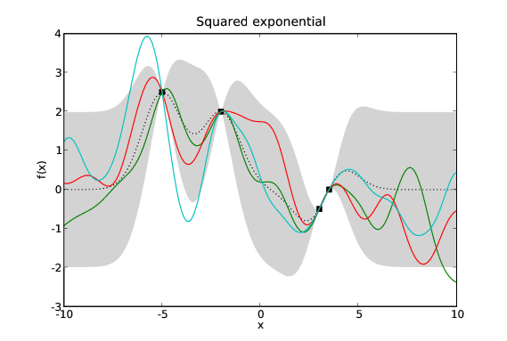
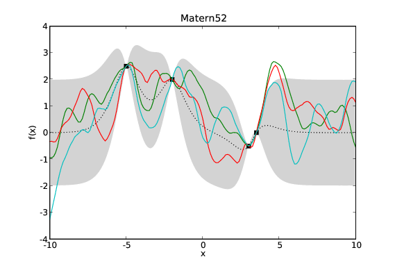
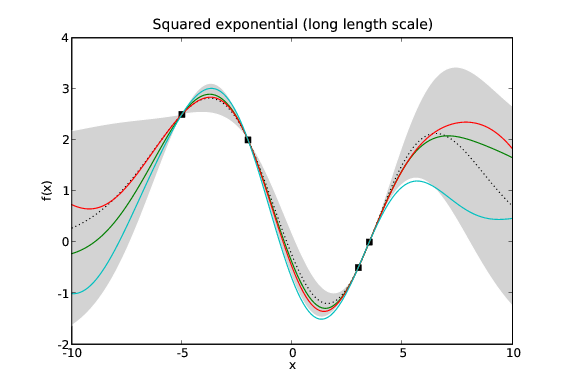
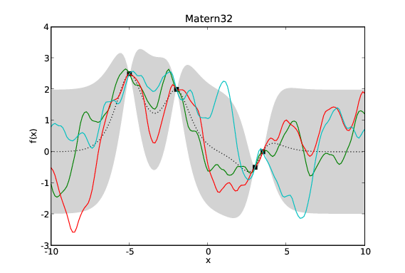
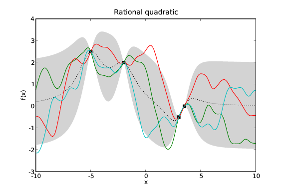
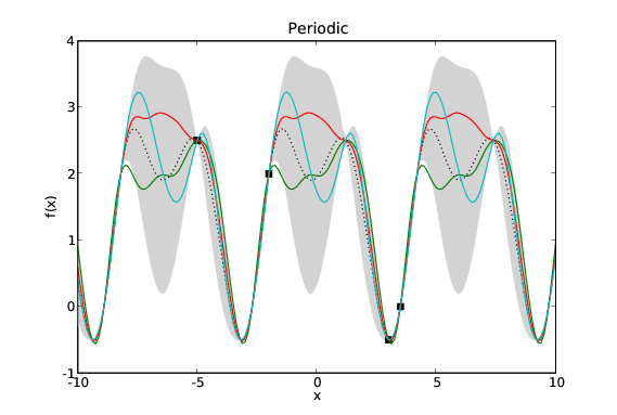
Samples drawn from GPs with the same data and different covariance functions. Typical samples from the posterior of GPs with different covariance functions have different characteristics. The periodic covariance function’s primary characteristic is self explanatory. The other covariance functions affect the smoothness of the samples in different ways.
The code to generate the above figures:
from numpy.random import seed
from infpy.gp import GaussianProcess, gp_1D_X_range, gp_plot_samples_from
from pylab import plot, savefig, title, close, figure, xlabel, ylabel
from infpy.gp import SquaredExponentialKernel as SE
from infpy.gp import Matern52Kernel as Matern52
from infpy.gp import Matern52Kernel as Matern32
from infpy.gp import RationalQuadraticKernel as RQ
from infpy.gp import NeuralNetworkKernel as NN
from infpy.gp import FixedPeriod1DKernel as Periodic
from infpy.gp import noise_kernel as noise

# seed RNG to make reproducible and close all existing plot windows
seed(2)
close('all')

#
# Part of X-space we will plot samples from
#
support = gp_1D_X_range(-10.0, 10.01, .125)

#
# Data
#
X = [[-5.], [-2.], [3.], [3.5]]
Y = [2.5, 2, -.5, 0.]

def plot_for_kernel(kernel, fig_title, filename):
  figure()
  plot([x[0] for x in X], Y, 'ks')
  gp = GaussianProcess(X, Y, kernel)
  gp_plot_samples_from(gp, support, num_samples=3)
  xlabel('x')
  ylabel('f(x)')
  title(fig_title)
  savefig('%s.png' % filename)
  savefig('%s.eps' % filename)

plot_for_kernel(
  kernel=Periodic(6.2),
  fig_title='Periodic',
  filename='covariance_function_periodic'
)

plot_for_kernel(
  kernel=RQ(1., dimensions=1),
  fig_title='Rational quadratic',
  filename='covariance_function_rq'
)

plot_for_kernel(
  kernel=SE([1]),
  fig_title='Squared exponential',
  filename='covariance_function_se'
)

plot_for_kernel(
  kernel=SE([3.]),
  fig_title='Squared exponential (long length scale)',
  filename='covariance_function_se_long_length'
)

plot_for_kernel(
  kernel=Matern52([1.]),
  fig_title='Matern52',
  filename='covariance_function_matern_52'
)

plot_for_kernel(
  kernel=Matern32([1.]),
  fig_title='Matern32',
  filename='covariance_function_matern_32'
)
Combining covariance functions and noisy data
Furthermore the point-wise product and sum of covariance functions are themselves covariance functions. In this way we can combine simple covariance functions to represent more complicated beliefs we have about our functions.
Normally we are modelling a system where we do not actually have access to the target values, \(y\), but only noisy versions of them, \(y+\epsilon\). If we assume \(\epsilon\) has a Gaussian distribution with variance \(\sigma_n^2\) we can incorporate this noise term into our covariance function. This requires that our noisy GP’s covariance function, \(k_{\textrm{noise}}(x_1,x_2)\) is aware of whether \(x_1\) and \(x_2\) are the same input as we may have two noisy measurements at the same point in \(\mathcal{X}\).
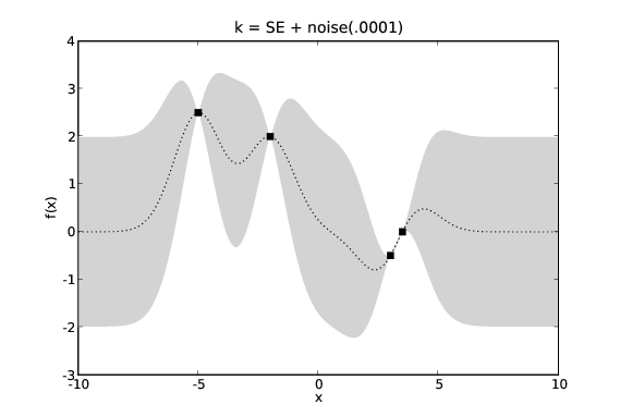
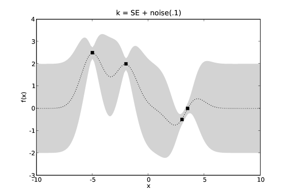
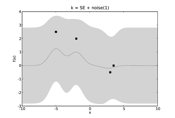
GP predictions with varying levels of noise. The covariance function is a squared exponential with additive noise of levels 0.0001, 0.1 and 1.
The code to generate the above figures:
from numpy.random import seed
from infpy.gp import GaussianProcess, gp_1D_X_range, gp_plot_prediction
from pylab import plot, savefig, title, close, figure, xlabel, ylabel
from infpy.gp import SquaredExponentialKernel as SE
from infpy.gp import noise_kernel as noise

# close all existing plot windows
close('all')

#
# Part of X-space we are interested in
#
support = gp_1D_X_range(-10.0, 10.01, .125)

#
# Data
#
X = [[-5.], [-2.], [3.], [3.5]]
Y = [2.5, 2, -.5, 0.]

def plot_for_kernel(kernel, fig_title, filename):
  figure()
  plot([x[0] for x in X], Y, 'ks')
  gp = GaussianProcess(X, Y, kernel)
  mean, sigma, LL = gp.predict(support)
  gp_plot_prediction(support, mean, sigma)
  xlabel('x')
  ylabel('f(x)')
  title(fig_title)
  savefig('%s.png' % filename)
  savefig('%s.eps' % filename)

plot_for_kernel(
  kernel=SE([1.]) + noise(.1),
  fig_title='k = SE + noise(.1)',
  filename='noise_mid'
)

plot_for_kernel(
  kernel=SE([1.]) + noise(1.),
  fig_title='k = SE + noise(1)',
  filename='noise_high'
)

plot_for_kernel(
  kernel=SE([1.]) + noise(.0001),
  fig_title='k = SE + noise(.0001)',
  filename='noise_low'
)
Learning covariance function parameters
Most of the commonly used covariance functions are parameterised. The parameters can be fixed if we are confident in our understanding of the problem. Alternatively we can treat them as hyper-parameters in our Bayesian inference task and optimise them through some technique such as maximum likelihood estimation or conjugate gradient descent.
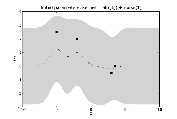
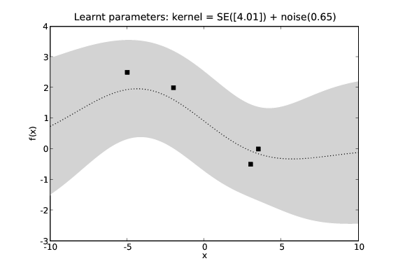
The effects of learning covariance function hyper-parameters. We see the predictions in the second figure seem to fit the data more accurately.
The code to generate the above figures:
from numpy.random import seed
from infpy.gp import GaussianProcess, gp_1D_X_range
from infpy.gp import gp_plot_prediction, gp_learn_hyperparameters
from pylab import plot, savefig, title, close, figure, xlabel, ylabel
from infpy.gp import SquaredExponentialKernel as SE
from infpy.gp import noise_kernel as noise

# close all existing plot windows
close('all')

#
# Part of X-space we are interested in
#
support = gp_1D_X_range(-10.0, 10.01, .125)

#
# Data
#
X = [[-5.], [-2.], [3.], [3.5]]
Y = [2.5, 2, -.5, 0.]

def plot_gp(gp, fig_title, filename):
  figure()
  plot([x[0] for x in X], Y, 'ks')
  mean, sigma, LL = gp.predict(support)
  gp_plot_prediction(support, mean, sigma)
  xlabel('x')
  ylabel('f(x)')
  title(fig_title)
  savefig('%s.png' % filename)
  savefig('%s.eps' % filename)

#
# Create a kernel with reasonable parameters and plot the GP predictions
#
kernel = SE([1.]) + noise(1.)
gp = GaussianProcess(X, Y, kernel)
plot_gp(
  gp=gp,
  fig_title='Initial parameters: kernel = SE([1]) + noise(1)',
  filename='learning_first_guess'
)

#
# Learn the covariance function's parameters and replot
#
gp_learn_hyperparameters(gp)
plot_gp(
  gp=gp,
  fig_title='Learnt parameters: kernel = SE([%.2f]) + noise(%.2f)' % (
    kernel.k1.params[0],
    kernel.k2.params.o2[0]
  ),
  filename='learning_learnt'
)