Examples

Here we give some examples of how to use infpy to use Gaussian processes models. We show how to

• examine the effects of different kernels
• model noisy data
• learn the hyperparameters of the model
• use periodic covariance functions

Data

We generate some noisy test data from a modulated sine using this script

import numpy, pylab, infpy.gp

# Generate some noisy data from a modulated sine curve
x_min, x_max = 10.0, 100.0
X = infpy.gp.gp_1D_X_range(x_min, x_max) # input domain
Y = 10.0 * numpy.sin(X[:,0]) / X[:,0] # noise free output
Y = infpy.gp.gp_zero_mean(Y) # shift so mean=0.
e = 0.03 * numpy.random.normal(size = len(Y)) # noise
f = Y + e # noisy output

# a function to save plots
def save_fig(prefix):
    "Save current figure in extended postscript and PNG formats."
    pylab.savefig('%s.png' % prefix, format='PNG')
    pylab.savefig('%s.eps' % prefix, format='EPS')
  
# plot the noisy data
pylab.figure()
pylab.plot(X[:,0], Y, 'b-', label='Y')
pylab.plot(X[:,0], f, 'rs', label='f')
pylab.legend()
save_fig('simple-example-data')
pylab.close()

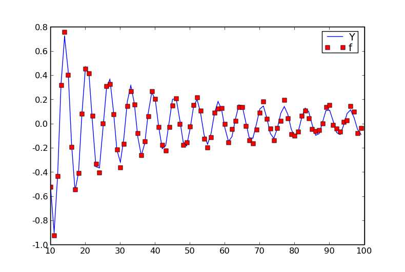
The \(f\)s are noisy observations of the underlying \(Y\)s. How can we model this using GPs?

Test different kernels

Using the following function as an interface to the infpy GP library

def predict_values(K, file_tag, learn=False):
    """
    Create a GP with kernel K and predict values.
    Optionally learn K's hyperparameters if learn==True.
    """
    gp = infpy.gp.GaussianProcess(X, f, K)
    if learn:
        infpy.gp.gp_learn_hyperparameters(gp)
    pylab.figure()
    infpy.gp.gp_1D_predict(gp, 90, x_min - 10., x_max + 10.)
    save_fig(file_tag)
    pylab.close()

we can test various different kernels to see how well they fit the data. For instance a simple squared exponential kernel with some noise

import infpy.gp.kernel_short_names as kernels
K = kernels.SE() + kernels.Noise(.1) # create a kernel composed of a squared exponential kernel and a small noise term
predict_values(K, ’simple-example-se’)

will generate

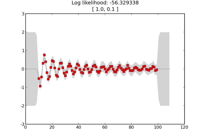
if we change the kernel so that the squared exponential term is given a shorter characteristic length scale

K = kernels.SE([.1]) + kernels.Noise(.1) # Try a different kernel with a shorter characteristic length scale
predict_values(K, ’simple-example-se-shorter’)

we will generate

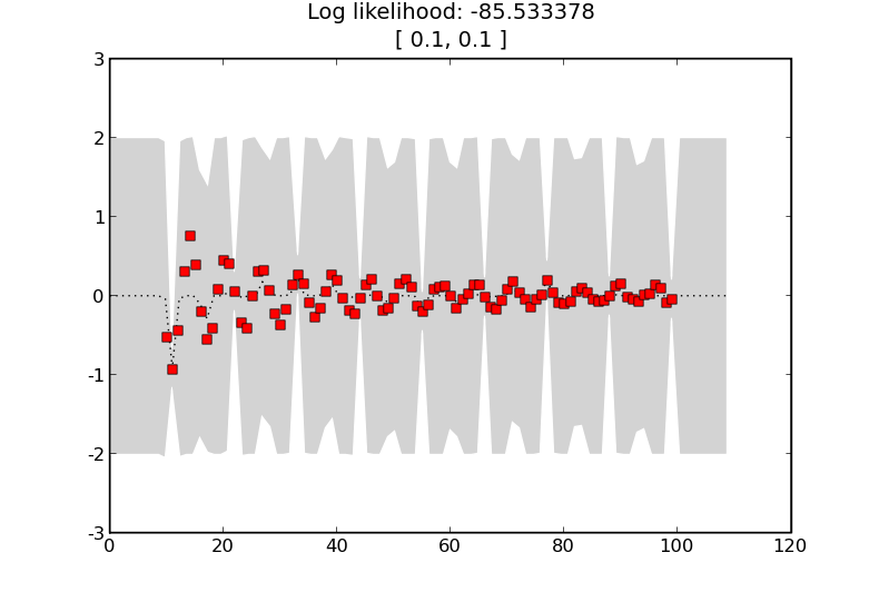
Here the shorter length scale means that data points are less correlated as the GP allows more variation over the same distance. The estimates of the noise between the training points is now much higher.

Effects of noise

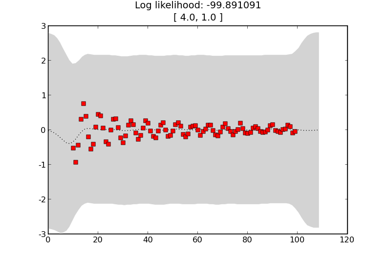
If we try a kernel with more noise

K = kernels.SE([4.]) + kernels.Noise(1.)
predict_values(K, ’simple-example-more-noise’)

we get the following estimates showing that the training data does not affect the predictions as much

Learning the hyperparameters

Perhaps we are really interested in learning the hyperparameters. We can acheive this as follows

K = kernels.SE([4.0]) + kernels.Noise(.1) # Learn kernel hyper-parameters
predict_values(K, ’simple-example-learnt’, learn=True)

and the result is

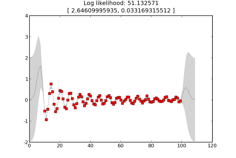
where the learnt length-scale is about 2.6 and the learnt noise level is about 0.03.

UK gas consumption example

We can apply these techniques with periodic covariance functions to UK gas consumption data from R.

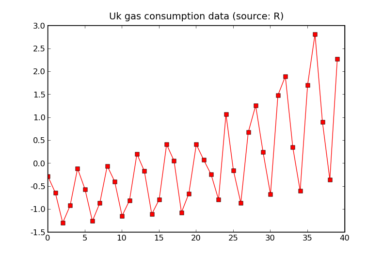
The data which has been shifted to have a mean of 0.

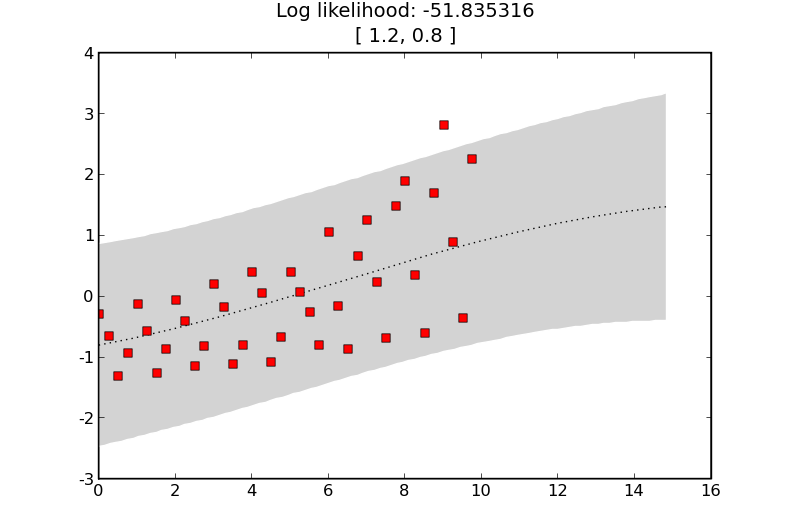
A GP incorporating some noise and a fixed long length scale squared exponential kernel.

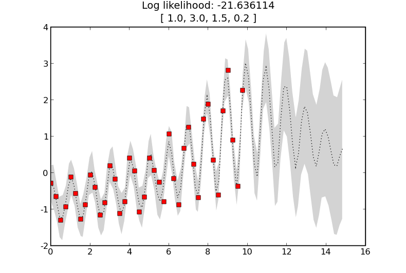
As before but with a periodic term.

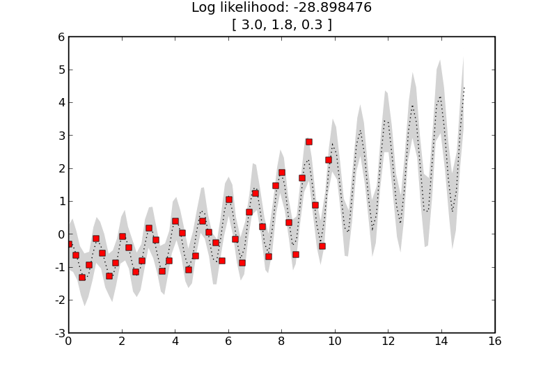
Now with a periodic term with a reasonable period.

Modulated sine example

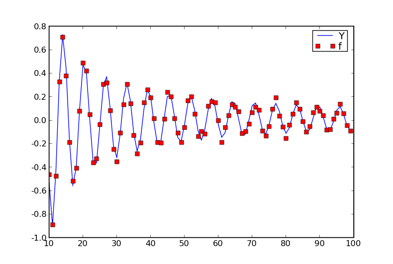
The data: a modulated noisy sine wave.

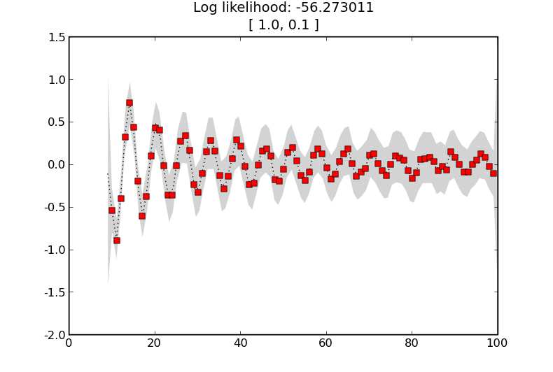
GP with a squared exponential kernel.

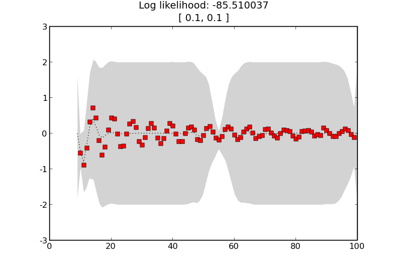
GP with a squared exponential kernel with a shorter length scale.

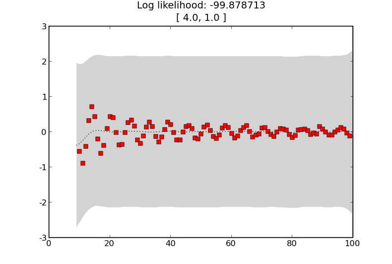
GP with a squared exponential kernel with a larger noise term.

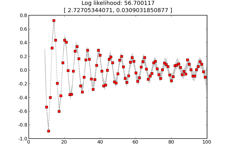
GP with a squared exponential kernel with learnt hyper-parameters. This maximises the likelihood.