User Guide

The easiest way to conduct an experiment is to use the GLAB application programming interface (API), which provides a simplified MATLAB-like interface to specify the experimental protocol and drive the computation of results. This section walks through an example use of this API.

Running an Experiment

We start by launching IPython, which is the recommended way to use Glimpse.

$ ipython --pylab

We then set up the environment:

>>> from glimpse.glab.api import *

>>> Verbose(True)

Here, we first import GLAB, and then ask that future commands log their activity to the console.

Note

Note that the “$” prefix used here denotes a command that is entered at the shell. The >>> denotes text that is submitted to the Python interpreter, or written as commands in a script. Lines without either marker indicate logging output.

The next step is to specify the experimental protocol and configure the model. We first tell Glimpse where to find the image corpora. The simplest way to achieve this is the SetCorpus command, which assumes one sub-directory per object class. That is, each of these sub-directories should contain images for only that object class. In this example, we have a corpus of images in a directory named “cats_and_dogs” with the following structure:

cats_and_dogs/
  cat/
    cat1.png
    cat2.png
    cat3.png
    cat4.png
  dog/
    dog1.png
    dog2.png
    dog3.png
    dog4.png

We tell Glimpse to use this corpus with the following command:

>>> SetCorpus('cats_and_dogs')
INFO:root:Reading class sub-directories from: cats_and_dogs
INFO:root:Reading images from class directories:
  ['cats_and_dogs/cat', 'cats_and_dogs/dog']

Here, the system reports that it has read the images for object classes “cat” and “dog” from disk.

Note

If you would like to learn about Glimpse without using your own image corpus, try using the SetCorpusByName() command.

Next, the model is configured with a set of (in this case 10) imprinted prototypes:

>>> ImprintS2Prototypes(10)
INFO:root:Using pool: MulticorePool
INFO:root:Learning 10 prototypes at 1 sizes from 4
  images by imprinting
Time: 0:00:01   |###############|   Speed: 3.07 unit/s
INFO:root:Learning prototypes took 1.304s

The first line of log output shows that images are being evaluated in parallel. Since we did not specify a training and testing split, the system has automatically chosen four (i.e., half) of the images for training and the remaining four for testing. The next line of log output confirms that the system imprinted 10 S2 prototypes, using the four images in the training set. (Here, prototypes are of 1 size, because the model uses only 7x7 prototypes by default. If we had configured the model to use 7x7 and 11x11 prototypes, for example, then we would have imprinted 10 prototypes at 7x7, and another 10 at 11x11, or 20 prototypes total.)

Finally, the model is used to extract features for each image, and the classifier is tested in the resulting feature space.

>>> EvaluateClassifier()
INFO:root:Computing C2 activation maps for 8 images
Time: 0:00:01   |###############|   Speed: 5.66 unit/s
INFO:root:Computing activation maps took 1.414s
INFO:root:Evaluating classifier on fixed train/test
  split on 8 images using 10 features from layer(s): C2
INFO:root:Training on 4 images took 0.003s
INFO:root:Classifier is Pipeline(learner=LinearSVC
  [...OUTPUT REMOVED...]
INFO:root:Classifier accuracy on training set is
  1.000000
INFO:root:Scoring on training set (4 images) took
  0.001s
INFO:root:Scoring on testing set (4 images) took 0.001s
INFO:root:Classifier accuracy on test set is 0.500000

The log output shows that the system is computing model activity through the C2 layer for all eight images in the corpus. Feature vectors are then constructed from C2 layer activity only, which provides 10 features per image (since we used 10 S2 prototypes). The classifier—which we can see is a linear SVM—is adapted to the training set, and then scored on both the training and test sets. In this case, accuracy was 100% on the training set, and 50% on the test set. See the GLAB API reference for the full set of available commands.

Command-Line Experiments

The experiment described above can also be run from the command line using the glab command. This command exposes much of the functionality of the API, but does so through comand-line arguments. To run the experiment above, we could enter the following at the command line (rather than the Python interpreter).

$ glab -v -c cats_and_dogs -p imprint -n 10 -E

This results in the same calls that were used in above, and thus should produce the same log output. Here, the -v flag enables the generation of log output, the -c flag specifies the image corpus, the -p and -n flags choose the prototype learning method and number of prototypes, and the -E flag evaluates the resulting feature vectors with a linear SVM classifier. The glab command has many more possible arguments, which are documented in the GLAB CLI reference.

Analyzing Results

Results can by analyzed in much the same way as an experiment is run. Using the GLAB API, we can first retrieve the set of images and their class labels:

>>> GetImagePaths()
array([
  'cats_and_dogs/cat/cat1.png',
  'cats_and_dogs/cat/cat2.png',
  'cats_and_dogs/cat/cat3.png',
  'cats_and_dogs/cat/cat4.png',
  'cats_and_dogs/dog/dog1.png',
  'cats_and_dog/dog/dog2.png',
  'cats_and_dog/dog/dog3.png',
  'cats_and_dog/dog/dog4.png'],
dtype='|S18')

>>> GetLabelNames()
array([
  'cat', 'cat', 'cat', 'cat',
  'dog', 'dog', 'dog', 'dog'],
dtype='|S3')

This means that the filenames and labels are stored as arrays. The “dtype” line can be ignored. It simply means that the values in that array are 18-character strings.

Model, Prototypes, and Activity Analysis

Information about the “extraction” phase of the experiment—i.e., how features were extracted from each image—is also available for analysis, which includes the model’s prototypes and parameters. The model parameters can be printed as follows:

>>> params = GetParams()

>>> params
Params(
  c1_kwidth = 11,
  c1_sampling = 5,
  c1_whiten = False,
  [...OUTPUT REMOVED...]
  s2_operation = 'Rbf',
  s2_sampling = 1,
  scale_factor = 1.189207115,
)

For example, this shows that an RBF activation function was used for the S2 layer (according to s2_operation), and that each scale band is \(2^{1/4}\) larger than the scale above it (according to scale_factor). The full set of parameters is documented here.

Note

The experiment’s model parameters can be edited with a graphical interface using SetParamsWithGui(). However, this must be done before the call to ImprintS2Prototypes() above.

If a set of S2 prototypes was used, they are available from the GetPrototype() command:

>>> prototype = GetPrototype(0)

>>> prototype.shape
(4, 7, 7)

>>> prototype
array([[[ 4.08234773e-03, 4.08234773e-03, ...,
          [...OUTPUT REMOVED...]
          4.65552323e-03, 5.46302684e-02 ]]],
      dtype=float32)

Output from the second command shows that each prototype is a seven-by-seven patch with four bands—i.e., a prototype is a three-dimensional array. The width of the patch is determined by the model parameters, as seen by the following:

>>> params.s2_kernel_widths
[7]

Remember that an S2 prototype is just a patch of C1 activity. Thus, the number of bands in a prototype is determined by the number of orientations used at the S1 and C1 layers. This can be confirmed as follows:

>>> params.s1_num_orientations
4

The number of available prototypes depends on the number that were learned. In our example, 10 prototypes were imprinted, which can be verified as:

>>> GetNumPrototypes()
10

As seen above, an S2 prototype is a somewhat complicated object to visualize, particularly in the form of text output. However, there are other ways to visualize a prototype. The simplest is to plot the activation at each band as a set of images, which we do here for the first prototype [1].

>>> gray()

>>> ShowPrototype(0)

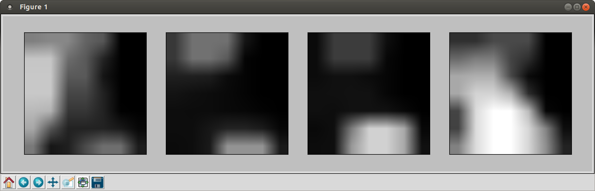
Figure 1: S2 prototype bands, with plots corresponding to edge orientations.

Note

Plotting in Glimpse requires the matplotlib library.

This results in a plot similar to that shown in Figure 1. Here, active locations are shown in white, while inactive locations are shown in black. These four plots correspond to the four edge orientations detected at S1. For reference, the S1 edge detectors [2] are shown as in Figure 2 using the following command:

>>> ShowS1Kernels()

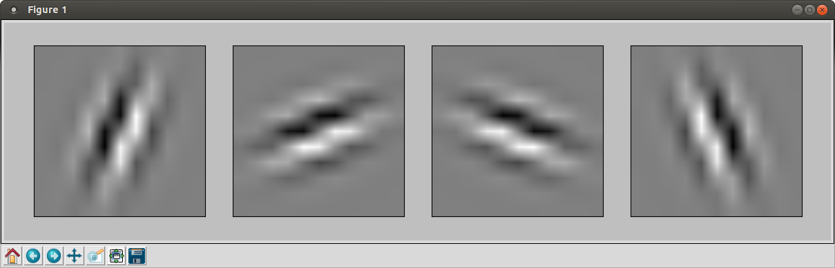
Figure 2: S1 edge detectors.

Unfortunately, the above visualization is not very intuitive. An alternative approach to visualizing an imprinted prototype is to plot the image patch from which the prototype was “imprinted”:

>>> AnnotateImprintedPrototype(0)

Note

To add a colorbar to this plot, just type:

>>> colorbar()

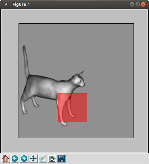
Figure 3: Chosen location for the imprinted S2 prototype.

The results are shown in Figure 3. Taken together, it is much easier to interpret the behavior of this prototype. We see that it was imprinted from the cat’s front leg, which contains a large amount of vertical energy and very little horizontal energy. This is reflected in the S2 prototype matrix, which shows light gray and white for the components corresponding to the two near-vertical detectors, and shows black for much of the components corresponding to the two near-horizontal detectors.

Additionally, we can investigate the model activity that was computed for various layers. Here, we visualize the activity of the S2 layer when the prototype in Figure 1 is applied to the image in Figure 3. We first need to know where the first prototype was imprinted, which is given by:

>>> image, scale, y, x = GetImprintLocation(0)

This returns the image and S2 location (including the scale band) for the imprinted prototype. Here, the image is specified by its index in the list of image paths, with other data organized in the same way. To plot the S2 activation for the first prototype on the image and scale from which it was imprinted, use:

>>> AnnotateS2Activity(image, scale, 0)

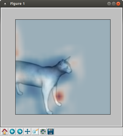
Figure 4: S2 response for the prototype visualized in Figure 1. For reference, the S2 activity is plotted on top of the image data.

This is shown for our expample in Figure 4, where active regions are shown in red and inactive regions are shown in blue. If the scale is larger than 2 or 3, the image data may be hard to recognize (as it has been down-sampled multiple times). In this case, try recreating the plot for smaller values of the scale argument.

A similar visualization as above is available for S1 and C1 activity as:

>>> AnnotateS1Activity(image, scale)

>>> AnnotateC1Activity(image, scale)

which should produce results similar to Figure 5 and Figure 6.

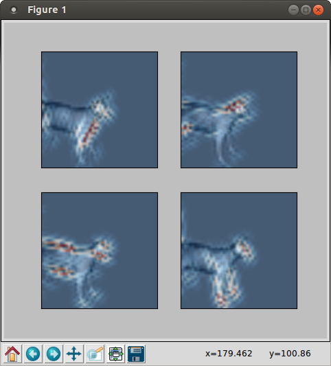
Figure 5: S1 response maps (enhanced for illustration).

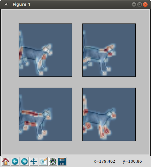
Figure 6: C1 response maps.

Classifier Analysis

In the final stage of an experiment, a classifier is evaluated on the feature vectors extracted by the model. The information about this stage is available via two functions: GetEvaluationLayers() and GetEvaluationResults(). First, we can verify that the classifier used an image representation based on C2 activity:

>>> GetEvaluationLayers()
['C2']

Information about the classifier’s performance can be given as:

>>> results = GetEvaluationResults()

>>> results.score_func
'accuracy'

>>> results.score
0.5

>>> results.training_score
1.0

The first result indicates that the classifier is evaluated based on accuracy, and the second result gives that accuracy on the set of test images. The last result gives the accuracy on the set of training images. The induced classifier can be retrieved as well:

>>> results.classifier
Pipeline(steps=[
   ('scaler', StandardScaler([...OUTPUT REMOVED...])
   ('learner', LinearSVC([...OUTPUT REMOVED...])
])

The per-image predictions made by the classifier are accessible by using:

>>> GetPredictions()
[('cats_and_dog/cat/cat3.png', 'cat', 'dog'),
 ('cats_and_dog/cat/cat4.png', 'cat', 'dog'),
 ('cats_and_dog/dog/dog1.png', 'dog', 'dog'),
 ('cats_and_dog/dog/dog2.png', 'dog', 'dog')]

>>> GetPredictions(training=True)
[('cats_and_dog/cat/cat3.png', 'cat', 'cat'),
 ('cats_and_dog/cat/cat4.png', 'cat', 'cat'),
 ('cats_and_dog/dog/dog1.png', 'dog', 'dog'),
 ('cats_and_dog/dog/dog2.png', 'dog', 'dog')]

The first call returned information about images in the test set, while the second call used the training images. Each entry of the results gives the image’s filename, its true label, and the label predicted by the classifier, respectively. In our example, the classifier predicted “dog” for all test images—thus achieving 50% accuracy—while correctly classifying all training images.

Finally, it may be useful during analysis to compute feature vectors for images outside the experiment’s corpus, which can be done using:

>>> features = GetImageFeatures('bird/bird1.png')
>>> features.shape
(1, 10)

This shows that our existing model with 10 S2 prototypes was used to extract 10 features from a single image. To extract features from several images at once, use:

>>> features = GetImageFeatures(['bird/bird1.png', 'bird/bird2.png'])
>>> features.shape
(2, 10)

[1]	Indexing in Python is zero-based, so the first prototype is at index zero.

[2]	We use the terms “prototype” and “kernel” somewhat interchangably.