Running the Face Recognition Experiments

To run the examples, just call the scripts from within the bin directory, e.g.:

$ ./bin/eigenface.py

If you installed the image database in another folder than Database, please give this directory as parameter to the script, e.g.:

$ ./bin/eigenface.py <AT&T_DATABASE_DIR>

There are three experiment scripts:

$ ./bin/eigenface.py
$ ./bin/gabor_graph.py
$ ./bin/dct_ubm.py

that perform more or less complicated face verification experiments using an unbiased evaluation protocol. Each experiment creates an ROC curve that contains the final verification result of the test. The generated files will be eigenface.pdf, gabor_graph.pdf and dct_ubm.pdf, respectively.

Since the complexity of the algorithms increase, the expected execution time of them differ a lot. While the eigenface experiment should be finished in a couple of seconds, the Gabor graph experiment could take some minutes, and the UBM/GMM model needs in the order of half an hour to compute.

Note

The example code that is presented here differ slightly from the code in the source files. Here, only the concepts of the functions should be clarified, while the source files contain code that is better arranged and computes faster.

In this small example, we use the bob.db.atnt database. This database is compatible with all other bob.db.verification.utils.Databases, so any other Databases that Implement the Database Interface can be used in a direct replacement of bob.db.atnt.

Overall Structure of an Experiment

All three examples have the same basic structure, which shows the simplicity of implementing any face recognition algorithm with the provided database interface. First, the bob.db.atnt.Database database interface is created, which will be be used to assure that we follow the default evaluation protocol of the database:

>>> db = bob.db.atnt.Database(original_directory = "...")

In total, there are four steps for each algorithm:

1. Training:

   Images from the training set are loaded (using the bob.example.faceverify.utils.load_images() function discussed below). Features from the training set are extracted and used to train the model.

   >>> training_files = db.training_files()
   >>> training_images = load_images(db, training_files) 
   >>> training_features = [extract_feature(image) for image in training_images]
   

2. Model Enrollment:

   Models are enrolled using features from several images for each model. The enroll_files are queried for each model separately:

   >>> model_ids = db.model_ids(groups = 'dev')
   >>> models = {}
   >>> for model_id in model_ids:
   ...   enroll_files = db.enroll_files(groups = 'dev', model_id = model_id)
   ...   enroll_images = load_images(db, enroll_files)
   ...   enroll_features = [extract_feature(enroll_image) for enroll_image in enroll_images]
   ...   models[model_id] = enroll(enroll_features)
   

3. Probe Feature Extraction:

   Probe features are extracted for all probe features. They are stored in a dictionary, using the File.id of the probe File object as keys:

   >>> probe_files = db.probe_files(groups = 'dev')
   >>> probe_images = load_images(db, probe_files) 
   >>> probes = {}
   >>> for i in range(len(probe_files)):
   ...   probe_id = probe_files[i].id
   ...   probes[probe_id] = extract_feature(probe_images[i])
   

4. Comparison of Model and Probe:

   Now, scores are computed by comparing the created models with the extracted probe features. Some of the protocols of our databases (e.g., the bob.db.banca database) require that each model is compared only to a model-specific sub-set of probes. Hence, for each model we have to query the database again. Finally, we need to know if the pair was a positive pair (i.e., when model and probe came from the same client), or negative (i.e., model and probe came from different clients):

   >>> positives = []
   >>> negatives = []
   >>> for model_id, model in models.items():
   ...   model_client_id = db.get_client_id_from_model_id(model_id)
   ...   model_probe_files = db.probe_files(groups = 'dev', model_id = model_id)
   ...   for probe_file in model_probe_files:
   ...     score = compare(model, probes[probe_file.id])
   ...     if model_client_id == probe_file.client_id:
   ...       positives.append(score)
   ...     else:
   ...       negatives.append(score)
   

5. Evaluation of Scores:

   Finally, the two sets of scores are used to evaluate the face recognition system, using functionality of the bob.measure package. Here, we compute the FAR and the FRR at the EER threshold and plot the ROC curve:

   >>> threshold = bob.measure.eer_threshold(negatives, positives)
   >>> FAR, FRR = bob.measure.farfrr(negatives, positives, threshold)
   >>> bob.measure.plot.roc(negatives, positives, CAR=True)
   [...]
   

   Note

   Here we plot the ROC curves with logarithmic FAR axis — to highlight the interesting part of the curve, i.e., where the FAR values are small.

Loading Data

To load the image data, I have implemented the generic bob.example.faceverify.utils.load_images() function:

bob.example.faceverify.utils.load_images(database, files, face_cropper=None, preprocessor=None)

Loads the original images for the given list of File objects.

Keyword Parameters:

database : bob.db.verification.utils.Database or derived from it

The database interface to query.

files : [bob.db.verification.utils.File] or derived from it

A list of File objects for which the images should be loaded.

face_cropper : bob.ip.base.FaceEyesNorm or None

If a face cropper is given, the face will be cropped using the eye annotations of the database.

preprocessor : function, object or None

If a preprocessor is given, it will be applied to the (cropped) faces.

This function is generic in the sense that:

1. it can read gray level and color images:

   >>> image = bob.io.base.load(filename) 
   >>> if len(image.shape) == 3:
   ...   gray_image = bob.ip.color.rgb_to_gray(image)
   

2. when eyes annotations are available, it can apply a face cropper bob.ip.base.FaceEyesNorm using the given eye positions, e.g.:

   >>> face_cropper = bob.ip.base.FaceEyesNorm(crop_size = (112,92), right_eye = (20,31), left_eye = (20,62))
   >>> cropped_image = face_cropper(gray_image, right_eye = (30,40), left_eye = (32, 60))
   

3. a preprocessor can be applied to the images, which is either a function or a class like bob.ip.base.TanTriggs that has the () operator (aka the __call__ function) overloaded:

   >>> preprocessor = bob.ip.base.TanTriggs()
   >>> preprocessed_image = preprocessor(cropped_image)
   

Finally, this function applies some or all of these steps on a list of images.

The Experiments

For the three implemented face recognition experiments, we have chosen different ways to preprocess the images, to train the system, to extract the features, to enroll the models, to extract the probes and to compare models and probes.

The Eigenface Example

The eigenface example follows the work-flow that is presented in the original paper Eigenfaces for Recognition [TP91] by Turk and Pentland. To train the eigenspace, the images from the training set are linearized (i.e., the pixels of an image are re-arranged to form a single vector):

>>> training_set = numpy.vstack([image.flatten() for image in training_images])

Afterwards, a bob.learn.linear.PCATrainer is used to compute the PCA subspace:

>>> pca_trainer = bob.learn.linear.PCATrainer()
>>> pca_machine, eigen_values = pca_trainer.train(training_set)

For some distance functions, the eigenvalues are needed, but in our example we just ignore them. Finally, the number of kept eigenfaces is limited to 5:

>>> pca_machine.resize(pca_machine.shape[0], 5)

After training, the model and probe images are loaded, linearized, and projected into the eigenspace using the trained pca_machine. A possible extract_feature (image) function could look like:

>>> pca_machine.forward(image.flatten())

The enrollment of the client is done by collecting all model feature vectors. The enroll(features) function is quite simple:

>>> def enroll(features):
...   return features

To compute the verification result, each model feature is compared to each probe feature by computing the scipy.spatial.distance.euclidean() distance. Finally, all scores of one model and one probe are averaged to get the final score for this pair, which would translate into a compare(model, probe) function like:

>>> score = 0.
>>> for model_feature in model:
...   score += scipy.spatial.distance.euclidean(model_feature, probe) 
>>> score /= len(model)

The final ROC curve of this experiment is:

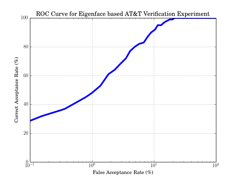
and the expected FAR and FRR performance is: FAR 9.15% and FRR 9% at threshold -9276.2

Note

Computing eigenfaces with such a low amount of training data is usually not an excellent idea. Hence, the performance in this example is relatively poor.

Gabor jet Comparison

A better face verification example uses Gabor jet features [WFKM97] . In this example we do not define a face graph, but instead we use the bob.ip.gabor.Jets at several grid positions in the image. In opposition to the Eigenface example above, here we preprocess the images with bob.ip.base.TanTriggs.

The Gabor graph extraction does not require a training stage. Therefore, in opposition to the eigenface example, the training images are not used in this example.

Instead, to extract Gabor grid graph features, it is sufficient to use:

>>> extractor = bob.ip.gabor.Graph((8,6), (104,86), (4,4))

that will create Gabor graphs with node positions from (8,6) to (104,86) with step size (4,4).

Note

The resolution of the images in the AT&T database is 92x112. Of course, there are ways to automatically get the size of the images, but for brevity we hard-coded the resolution of the images.

Now, the Gabor graph features can be extracted from the model and probe images:

>>> gabor_wavelet_transform = bob.ip.gabor.Transform()
>>> trafo_image = gabor_wavelet_transform.transform(preprocessed_image)
>>> model_graph = extractor.extract(trafo_image)

For model enrollment, as above we simply collect all enrollment features. To compare the Gabor graphs, several methods can be applied. Again, many choices for the Gabor jet comparison exist, here we take a novel Gabor phase based bob.ip.gabor.Similarity function [GHW12]:

>>> similarity_function = bob.ip.gabor.Similarity("PhaseDiffPlusCanberra", gabor_wavelet_transform)

Since we have several local features, we can exploit this fact. In the compare(model, probe) function, we compute the similarity between the probe feature at this position and all model features and take the maximum value for each grid position:

>>> for gabor_jet_index in range(len(probe_feature)):
...   scores = []
...   for model_feature_index in range(len(model)):
...     scores.append(SIMILARITY_FUNCTION(model[model_feature_index][gabor_jet_index], probe_feature[gabor_jet_index]))
...   score += max(scores)
>>> score /= len(probe_feature)

Since this method is better for suited for small image databases, the resulting verification rates are better. The expected ROC curve is:

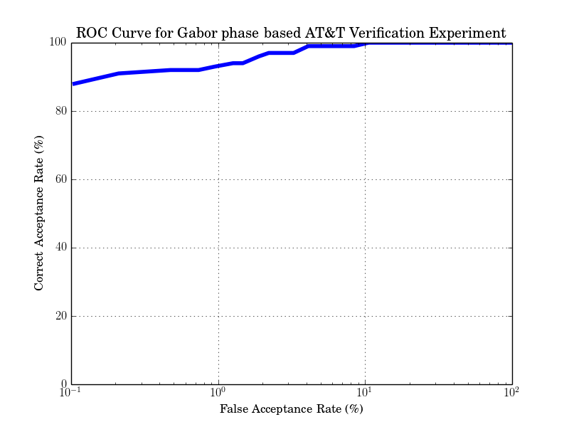
while the expected verification result is: FAR 3% and FRR 3% at distance threshold 0.5912

The UBM/GMM modeling of DCT Blocks

The last example shows a quite complicated, but successful algorithm. Again, images are preprocessed with bob.ip.base.TanTriggs. The first step is the feature extraction of the training image features and the collection of them in a 2D array. In this experiment we will use Discrete Cosine Transform (DCT) block features using bob.ip.base.DCTFeatures [MM09]:

>>> dct_extractor = bob.ip.base.DCTFeatures(45, (12, 12), (11, 11))
>>> features = dct_extractor(preprocessed_image)

Hence, from every image, several DCT block features are extracted independently. All these features are mixed together to build the training set:

>>> training_set = numpy.vstack(training_features)

With these training features, a universal background model (UBM) is computed [RQD00]. It is a Gaussian Mixture Model (GMM) that holds information about the overall distribution of DCT features in facial images. The UBM model is trained using a bob.learn.misc.KMeansTrainer to estimate the means of the Gaussians:

>>> kmeans_machine = bob.learn.em.KMeansMachine(...)
>>> kmeans_trainer = bob.learn.em.KMeansTrainer()
>>> bob.learn.em.train(kmeans_trainer, kmeans, training_set)

Afterward, the UBM is initialized with the results of the k-means training:

>>> ubm = bob.learn.em.GMMMachine(...)
>>> ubm.means = kmeans_machine.means
>>> [variances, weights] = kmeans_machine.get_variances_and_weights_for_each_cluster(training_set)
>>> ubm.variances = variances
>>> ubm.weights = weights

and a bob.learn.em.ML_GMMTrainer is used to compute the actual UBM model:

>>> trainer = bob.learn.em.ML_GMMTrainer()
>>> trainer.train(ubm, training_set)

After UBM training, the next step is the model enrollment. Here, a separate GMM model is generated by shifting the UBM towards the mean of the model features [MM09]. For that purpose, a bob.learn.misc.MAP_GMMTrainer is used:

>>> gmm_trainer = bob.learn.em.MAP_GMMTrainer()
>>> enroll_set = numpy.vstack(enroll_features)
>>> model_gmm = bob.learn.em.GMMMachine(ubm)
>>> bob.learn.em.train(gmm_trainer, model_gmm, model_feature_set)

Also the probe image need some processing. First, of course, the DCT features are extracted. Afterward, the bob.learn.misc.GMMStats statistics for each probe file are generated:

>>> probe_set = numpy.vstack([probe_feature])
>>> gmm_stats = bob.learn.em.GMMStats()
>>> ubm.acc_statistics(probe_dct_blocks, gmm_stats)

Finally, the scores for the probe files are computed using the bob.learn.misc.linear_scoring() function:

>>> score = bob.learn.em.linear_scoring([model], ubm, [probe_stats])[0,0]

Again, the evaluation of the scores is identical to the previous examples. The expected ROC curve is:

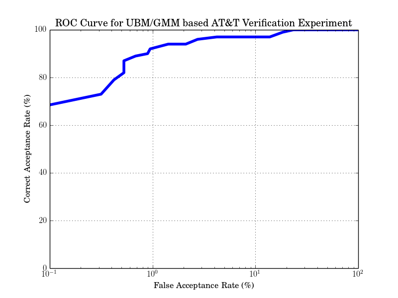
The expected result is: FAR 3.15% and FRR 3% at distance threshold 2301.58

[TP91]

Matthew Turk and Alex Pentland. Eigenfaces for recognition. Journal of Cognitive Neuroscience, 3(1):71-86, 1991.

[WFKM97]

Wiskott, J.-M. Fellous, N. Krüger and C.v.d. Malsburg. Face recognition by elastic bunch graph matching. IEEE Transactions on Pattern Analysis and Machine Intelligence, 19:775-779, 1997.

[GHW12]

Manuel Günther, Dennis Haufe, Rolf P. Würtz. Face recognition with disparity corrected Gabor phase differences. In Artificial Neural Networks and Machine Learning, 411-418, 2012.

[MM09]

(1, 2) Chris McCool and Sébastien Marcel. Parts-based face verification using local frequency bands. In proceedings of IEEE/IAPR international conference on biometrics. 2009.

[RQD00]

D.A. Reynolds, T.F. Quatieri, and R.B. Dunn. Speaker verification using adapted gaussian mixture models. Digital Signal Processing, 10(1-3):19–41, 2000.