Getting started
Before all examples below, it’s easier to get everything from audiolazy namespace:
from audiolazy import *
All modules starts with “lazy_”, but their data is already loaded in the main namespace. These two lines of code do the same thing:
from audiolazy.lazy_stream import Stream
from audiolazy import Stream
Endless iterables with operators (be careful with loops through an endless iterator!):
>>> a = Stream(2, -2, -1) # Periodic
>>> b = Stream(3, 7, 5, 4) # Periodic
>>> c = a + b # Elementwise sum, periodic
>>> c.take(15) # First 15 elements from the Stream object
[5, 5, 4, 6, 1, 6, 7, 2, 2, 9, 3, 3, 5, 5, 4]
And also finite iterators (you can think on any Stream as a generator with elementwise operators):
>>> a = Stream([1, 2, 3, 2, 1]) # Finite, since it's a cast from an iterable
>>> b = Stream(3, 7, 5, 4) # Periodic
>>> c = a + b # Elementwise sum, finite
>>> list(c)
[4, 9, 8, 6, 4]
LTI Filtering from system equations (Z-transform). After this, try summing, composing, multiplying ZFilter objects:
>>> filt = 1 - z ** -1 # Diff between a sample and the previous one
>>> filt
1 - z^-1
>>> data = filt([.1, .2, .4, .3, .2, -.1, -.3, -.2]) # Past memory has 0.0
>>> data # This should have internally [.1, .1, .2, -.1, -.1, -.3, -.2, .1]
<audiolazy.lazy_stream.Stream object at ...>
>>> data *= 10 # Elementwise gain
>>> [int(round(x)) for x in data] # Streams are iterables
[1, 1, 2, -1, -1, -3, -2, 1]
>>> data_int = filt([1, 2, 4, 3, 2, -1, -3, -2], zero=0) # Now zero is int
>>> list(data_int)
[1, 1, 2, -1, -1, -3, -2, 1]
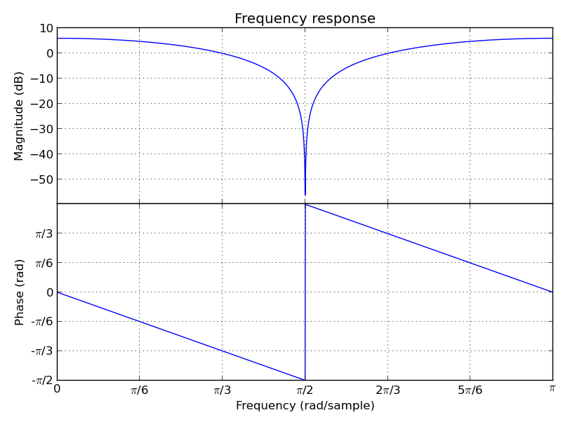
LTI Filter frequency response plot (needs MatPlotLib):
(1 + z ** -2).plot().show()
The matplotlib.figure.Figure.show method won’t work unless you’re
using a newer version of MatPlotLib (works on MatPlotLib 1.2.0), but you still
can save the above plot directly to a PDF, PNG, etc. with older versions
(e.g. MatPlotLib 1.0.1):
(1 + z ** -2).plot().savefig("my_plot.pdf")
On the other hand, you can always show the figure using MatPlotLib directly:
from matplotlib import pyplot as plt # Or "import pylab as plt"
filt = 1 + z ** -2
fig1 = filt.plot(plt.figure()) # Argument not needed on the first figure
fig2 = filt.zplot(plt.figure()) # The argument ensures a new figure
plt.show()
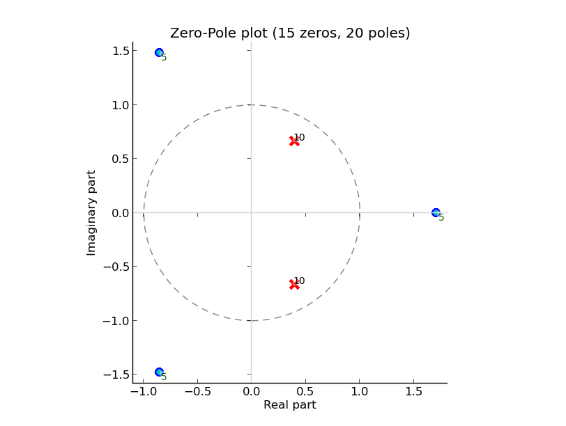
CascadeFilter instances and ParallelFilter instances are lists of filters with the same operator behavior as a list, and also works for plotting linear filters. Constructors accepts both a filter and an iterable with filters. For example, a zeros and poles plot (needs MatPlotLib):
filt1 = CascadeFilter(0.2 - z ** -3) # 3 zeros
filt2 = CascadeFilter(1 / (1 -.8 * z ** -1 + .6 * z ** -2)) # 2 poles
# Here __add__ concatenates and __mul__ by an integer make reference copies
filt = (filt1 * 5 + filt2 * 10) # 15 zeros and 20 poles
filt.zplot().show()
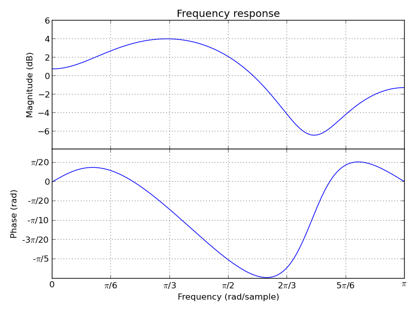
Linear Predictive Coding (LPC) autocorrelation method analysis filter frequency response plot (needs MatPlotLib):
lpc([1, -2, 3, -4, -3, 2, -3, 2, 1], order=3).plot().show()
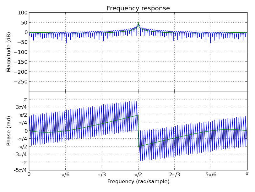
Linear Predictive Coding covariance method analysis and synthesis filter, followed by the frequency response plot together with block data DFT (MatPlotLib):
>>> data = Stream(-1., 0., 1., 0.) # Periodic
>>> blk = data.take(200)
>>> analysis_filt = lpc.covar(blk, 4)
>>> analysis_filt
1 + 0.5 * z^-2 - 0.5 * z^-4
>>> residual = list(analysis_filt(blk))
>>> residual[:10]
[-1.0, 0.0, 0.5, 0.0, 0.0, 0.0, 0.0, 0.0, 0.0, 0.0]
>>> synth_filt = 1 / analysis_filt
>>> synth_filt(residual).take(10)
[-1.0, 0.0, 1.0, 0.0, -1.0, 0.0, 1.0, 0.0, -1.0, 0.0]
>>> amplified_blk = list(Stream(blk) * -200) # For alignment w/ DFT
>>> synth_filt.plot(blk=amplified_blk).show()
AudioLazy doesn’t need any audio card to process audio, but needs PyAudio to play some sound:
rate = 44100 # Sampling rate, in samples/second
s, Hz = sHz(rate) # Seconds and hertz
ms = 1e-3 * s
note1 = karplus_strong(440 * Hz) # Pluck "digitar" synth
note2 = zeros(300 * ms).append(karplus_strong(880 * Hz))
notes = (note1 + note2) * .5
sound = notes.take(int(2 * s)) # 2 seconds of a Karplus-Strong note
with AudioIO(True) as player: # True means "wait for all sounds to stop"
  player.play(sound, rate=rate)
See also the docstrings and the “examples” directory at the github repository for more help. Also, the huge test suite might help you understanding how the package works and how to use it.